Computational Approaches to Understanding Subduction Zone Geodynamics, Surface Heat Flow, and the Metamorphic Rock Record

Buchanan C. Kerswell

26 May, 2023

Dedication

To my mentors, colleagues, friends, and loved ones who take special interests in my life.

Acknowledgment

This work was only possible through the efforts of many individuals. My advisor, Dr. Matthew Kohn, deserves special recognition for his contributions, mentorship, and relentless support during the course of my studies. Special thanks to my committee members, Dr. H.P. Marshall, Dr. C.J. Northrup, Dr. Philippe Agard. Thanks to Dr. Steve Utych who served as the Graduate College Representative for Boise State University. Dr. Taras Gerya and the Geophysical Fluid Dynamics group at the Institut für Geophysik, ETH Zürich, generously offered their high-performance computing resources, invaluable instruction, discussion, and support on the numerical modelling methods, and many free meals in Zürich. Additional high-performance computing support was provided by the Research Computing Department at Boise State University. Thanks to Dr. D. Hasterok for providing references and guidance on citing the large dataset in chapter three. Special thanks to Dr. Philippe Agard, Dr. Laetitia Le Pourhiet, and graduate students at Sorbonne Université for their incredible expertise and showing me the best of summertime Paris. Thanks to many anonymous reviewers, graduate students, and colleagues for helpful comments on technical aspects of each chapter. My deep appreciation of metamorphic rocks and Alpine geology was formed thanks to outstanding field excursions expertly guided by EFIRE and ZiP graduate students, faculty, and affiliates. I am especially grateful to Dr. Sarah Penniston-Dorland and Dr. Maureen Feinman for their tireless efforts in organizing those excursions. Funding for this work was provided by the National Science Foundation grant OIA1545903 awarded to Dr. Matthew Kohn, Dr. Sarah Penniston-Dorland, and Dr. Maureen Feineman. Datasets and code for reproducing this research are available on GitHub.

Abstract

PT estimates from exhumed HP metamorphic rocks and global surface heat flow observations evidently encode information about subduction zone thermal structure and the nature of mechanical and chemical processing of subducted materials along the interface between converging plates. Previous work demonstrates the possibility of decoding such geodynamic information by comparing numerical geodynamic models with empirical observations of surface heat flow and the metamorphic rock record. However, ambigous interpretations can arise from this line of inquiry with respect to thermal gradients, plate coupling, and detachment and recovery of subducted materials. This dissertation applies a variety of computational techniques to explore changes in plate interface behavior among subduction zones from large numerical and empirical datasets. First, coupling depths for 17 modern subduction zones are predicted after observing mechanical coupling in 64 numerical geodynamic simulations. Second, upper-plate surface heat flow patterns are assessed by applying two methods of interpolation to thousands of surface heat flow observations near subduction zone segments. Third, PT distributions of over one million markers traced from the previous set of 64 subduction simulations are compared with hundreds of empirical PT estimates from the rock record to assess the effects of thermo-kinematic boundary conditions on detachment and recovery of rock along the plate interface. These studies conclude the following. Mechanical coupling between plates is primarily controlled by the upper plate lithospheric thickness, with marginal responses to other thermo-kinematic boundary conditions. Upper-plate surface heat flow patterns are highly variable within and among subduction zone segments, suggesting both uniform and nonuniform subsurface thermal structure and/or geodynamics. Finally, PT distributions of recovered markers show patterns consistent with trimodal detachment (recovery) of rock from distinct depths coinciding with the continental Moho at ~35-40 km, the onset of plate coupling at ~80 km, and an intermediate recovery mode around ~55 km. Together, this work identifies important biases in geodynamic numerical models (insufficient implementation of recovery mechanisms and/or heat generation/transfer), surface heat flow observations (poor spatial coverage and/or oversampling of specific regions), and petrologic datasets (selective sampling of metamorphic rocks amenable to petrologic modelling techniques) that, if addressed, could significantly improve the current understandings of subduction interface behavior.

1 Introduction

As noted by Gerya (2014), a scarcity of observational constraints through time and space makes the study of geodynamics on Earth extraordinarily challenging (Figure 1.1). Fortunately, application of various computational approaches—simulation, interpolation, and applied statistics (machine learning)—enable geodynamic inquiry despite sparse datasets. This dissertation leverages the above computational methods to investigate a fundamental component of Plate Tectonic theory, subduction.

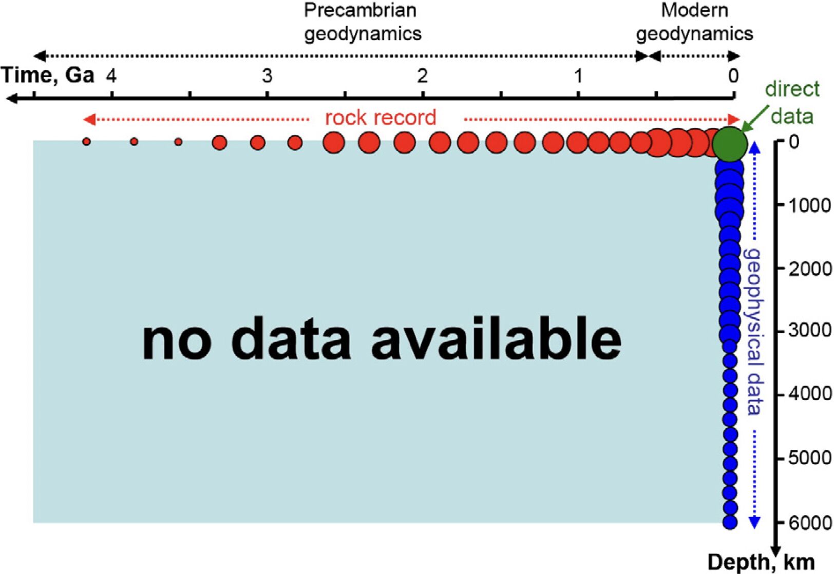
Figure 1.1: The Geodynamicist’s dilemma. Time-depth diagram representing the data availability on Earth. The rock record (red circles) encodes information about geodynamic processes throughout Earth’s history, but only within approximately 100 km of Earth’s surface. Geophysical data (blue circles) provide images of Earth’s deep interior, but only since the 20th century CE (or 10\(^{-7}\) Ga). Direct observations (green circle) are limited to the present-day surface. Size of the circles represents the abundance of available data. Reprinted from Gerya (2014) with permission.

Subduction occurs when two lithospheric plates converge and the denser plate subducts beneath the other at a subduction zone. Subduction zones drive many geodynamic phenomena, including plate motions, seismicity, metamorphism, volatile flux, volcanism, and crustal deformation (Čížková & Bina, 2013; Gao & Wang, 2017; Gonzalez et al., 2016; Grove et al., 2012; Hacker et al., 2003; Hirauchi et al., 2010; Peacock, 1990, 1991, 1993, 1996; Peacock & Hyndman, 1999; van Keken et al., 2011). These phenomena are largely defined by plate motions and mechanical behavior along the interface between the subducting plate and overriding (upper) plate (Furukawa, 1993; Peacock et al., 1994; Peacock, 1996). Important thermo-kinematic boundary conditions exerting first-order control on subduction zone geodynamics (plate velocity, subduction angle, plate thickness, sediment thickness, crustal structure, subduction duration, and others) vary considerably among presently active subduction zones worldwide (e.g. Syracuse et al., 2010; Syracuse & Abers, 2006).

Intuition suggests diverse thermo-kinematic boundary conditions for various subduction zone systems should influence mechanical behavior differently along the plate interface. Yet previous work comparing surface heat flow with numerical simulations of subduction argues for rather uniform depths of plate coupling among subduction zones (Furukawa, 1993; Wada et al., 2008; Wada & Wang, 2009) and implies some aspects of subduction zone mechanics are minimally affected by thermo-kinematic boundary conditions. Compounding the ambiguity are global compilations of PT estimates from exhumed HP metamorphic rocks that imply detachment of subducting material is either rather continuous along the plate interface (Agard et al., 2018; Penniston-Dorland et al., 2015) or discontinuous (Agard et al., 2009, 2016; Groppo et al., 2016; Monie & Agard, 2009; Plunder et al., 2015). Thus, the spatial variability (with depth and along strike) of plate interface mechanics remains largely unconstrained and difficult to quantify.

This dissertation is motivated by the following question. How can spatial variations in plate interface mechanics be evaluated across a range of subduction zones with currently available petrologic and geophysical datasets? Each chapter focuses on quantifying an aspect of subduction zone mechanics using different computational approaches and datasets.

Chapter 2 numerically simulates oceanic-continental subduction across a range of thermo-kinematic boundary conditions. Plate coupling is observed after 10 Ma and multivariate linear regression is then used to formulate an expression for estimating coupling depth. The expression requires estimates for upper-plate thickness, which can be inverted from surface heat flow. Average upper-plate surface heat flow for 13 presently active subduction zones yield a narrow distribution of coupling depths.

Chapter 3 takes a closer look surface heat flow by quantifying its spatial variability across large adjacent regions (sectors) in the upper-plate. Two interpolations methods, Kriging and Similarity, are compared to assess differences in their surface heat flow predictions near 13 subduction zone segments. Kriging and Similarity accuracies are comparable on average and both approaches show lateral (along strike) surface heat flow variability in the upper-plate. Discontinuous upper-plate surface heat flow implies nonuniform thermal structure and/or discontinuous geodynamics.

Finally, Chapter 4 applies machine learning techniques to recognize detachment of subducting markers (representing rock fragments) from the numerical simulations in Chapter 2. A large (119,146) PT dataset of recovered markers is compared across numerical experiments and with global compilation of PT estimates for rocks exhumed from subduction zones (the rock record, Agard et al., 2018; Penniston-Dorland et al., 2015). Marker PT distributions are distinct from the rock record for most numerical simulations, except for slowly-converging systems (40 km/Ma) with young oceanic plates (\(\leq\) 55 Ma) and thin upper-plate lithospheres. A sizeable gap in marker recovery around 2 GPa and 550 ˚C, closely coinciding with the highest density region of natural samples, implies certain biases may be affecting numerical geodynamic models, the rock record, or both.

2 Effects of Thermo-Kinematic Boundary Conditions on Plate Coupling in Subduction Zones

Abstract

Deep mechanical coupling between converging plates is implicated in dynamic plate motions, crustal deformation, seismic cycles, arc magmatism, detachment (recovery) of subducting material, and is considered a key feature of subduction zone geodynamics. This study uses two-dimensional numerical simulations of oceanic-continental convergent margins to investigate effects of thermo-kinematic boundary conditions on coupling—specifically focusing on thermal parameter (\(\Phi\)) and upper-plate thickness. Numerical simulations implement coupling by including the metamorphic (de)hydration reaction \(antigorite \Leftrightarrow olivine + orthopyroxene + H_{2}O\) in the upper-plate mantle. Visualizing PT-strain fields show thermal feedbacks regulating coupling depth dynamically with strong responses to upper-plate thickness and weak responses to \(\Phi\). The results imply estimation of coupling depth is possible by inverting upper-plate thickness from surface heat flow. Moreover, surface heat flow sampled from the backarc region near 17 presently active subduction zones imply uniform upper-plate thickness, and thus uniform coupling depths among subduction zones.

2.1 Introduction

Subduction geodynamics are largely defined by plate motions and mechanical behavior along the plate interface. For example, a transition from mechanically decoupled (plates moving differentially with respect to each other) to coupled plates (plates moving with the same local velocity) dramatically increases temperature by inducing mantle circulation in the upper-plate asthenospheric mantle (Peacock et al., 1994; Peacock, 1996). Observations from numerical simulations and forearc surface heat flow imply coupling transitions occur globally within a narrow range of depths in modern subduction zones (70-80 km). Further, coupling appears essentially unresponsive to diverse thermo-kinematic boundary conditions, including oceanic plate age, convergence velocity, and subduction geometry (Furukawa, 1993; Wada et al., 2008; Wada & Wang, 2009). While uniform coupling depths among subduction zones are inferred from numerical simulations and surface heat flow, this phenomenon remains curious and unconfirmed to a large extent. To understand subduction zone geodynamics, it is essential to understand why modern subduction zones appear to achieve similar coupling depths despite differences in their physical characteristics.

Notwithstanding, many numerical geodynamic models use coupling depths of 70-80 km as a boundary condition (Abers et al., 2017; Currie et al., 2004; Gao & Wang, 2014; Syracuse et al., 2010; van Keken et al., 2011, 2018; Wada et al., 2012; Wilson et al., 2014), although not exclusively (e.g. 40-56 km, England & Katz, 2010; Peacock, 1996). Similar coupling depths among subduction zones is an attractive hypothesis for at least two reasons. First, it helps explain a relatively narrow range of depths to subducting oceanic plates beneath volcanic arcs (England et al., 2004; Syracuse & Abers, 2006) as mechanical coupling is expected to be closely associated with the onset of flux melting. Second, mechanical coupling is required to detach crustal fragments from the subducting plate (Agard et al., 2016), so uniform coupling depths may also help explain why maximum pressures recorded by subducted oceanic material worldwide is \(\leq\) 2.3-2.5 GPa (roughly 80 km, Agard et al., 2009, 2018).

The location and extent of mechanical coupling along the plate interface is implicated in myriad geodynamic phenomena, including seismicity, metamorphism, volatile flux, volcanism, plate motions, and crustal deformation (Čížková & Bina, 2013; Gao & Wang, 2017; Gonzalez et al., 2016; Grove et al., 2012; Hacker et al., 2003; Hirauchi et al., 2010; Peacock, 1990, 1991, 1993, 1996; Peacock & Hyndman, 1999; van Keken et al., 2011). Consequently, the mechanics of coupling have been extensively studied and discussed. Coupling fundamentally depends on the strength (viscosity) of materials above, within, and below the plate interface. Water flux from compaction and dehydration of hydrous minerals with increasing PT forms layers of low viscosity sheet silicates near the plate interface. Transmission of shear stress between plates is inhibited by formation of talc and serpentine in the shallow upper-plate mantle (Peacock & Hyndman, 1999). Lack of traction along the interface, combined with cooling from the subducting plate surface, ensures a positive feedback between hydrous mineral formation and mechanical decoupling. Experimentally determined flow laws, petrologic observations, and geophysical observations all support the plausibility of this conceptual model of subduction interface behavior (e.g. Agard et al., 2016, 2018; Gao & Wang, 2014; Peacock & Hyndman, 1999).

Experimental control over important thermo-kinematic boundary conditions make geodynamic numerical simulations essential for investigating such complex geodynamic environments. Wada & Wang (2009) previously investigated the effects of \(\Phi\) on coupling depths by numerically simulating 17 presently active subduction zones. Among other thermo-kinematic boundary conditions, their models specify convergence rate, subduction geometry, thermal structure of oceanic- and overriding-plates, and degree of coupling along the subduction interface. Notably, their experiments control for interface rheology and discriminate best-fit coupling depths based on observed forearc surface heat flow.

This study similarly specifies thermo-kinematic boundary conditions to numerically simulate the range of modern subduction zone systems, but regulates interface rheology dynamically by implementing metamorphic reactions that respond to evolving PT-strain fields. Subduction geometry and coupling depth are not fully determined features, in other words, but spontaneous model outcomes within the range of specified boundary conditions discussed in Section 2.2. As in previous studies (e.g. Ruh et al., 2015), rheological effects of the dehydration reaction \(antigorite \Leftrightarrow olivine + orthopyroxene + H_{2}O\) are implemented to drive mechanical coupling. An abrupt viscosity increase accompanies antigorite (serpentine) destabilization, thereby inducing mechanical coupling, as defined by empirically-determined flow laws used in the numerical experiments.

This chapter focuses on two fundamental questions. How does coupling depth respond to \(\Phi\) and upper-plate thickness? And how stable is coupling depth through time? First, 64 convergent margins with variable upper-plate thickness and \(\Phi\) are numerically simulated and mechanical plate coupling is observed. Thermal feedbacks within the system are visualized in terms of mantle temperature, viscosity, and velocity fields and coupling depth responses to a range of \(\Phi\) and upper-plate thickness are quantified using multivariate linear regression. Three different regression models are then used to estimate coupling depths for 17 presently active subduction zones. Coupling depth estimates are narrowly distributed, regardless of regression model form. Finally, implications and questions regarding uniformity among subduction zones in terms of surface heat flow, upper-plate thickness, and coupling depth are discussed.

2.2 Numerical Modelling Methods

This study simulates converging oceanic-continental plates, where an ocean basin is being consumed by subduction at a continental margin (Figure 2.1). Initial conditions are modified from previous numerical experiments of active margins (Gorczyk et al., 2007; Sizova et al., 2010) using the code I2VIS (Gerya & Yuen, 2003), although plate coupling was not the focus of their studies. An identical rheologic model with identical material properties (Table 2.1), and a identical hydration/melt model (Table A.4 & Appendix A.3) to Sizova et al. (2010) are implemented. However, the version of I2VIS in this study differs from Sizova et al. (2010) in its initial setup, overall dimension, resolution, continental geotherm, dehydration model, and left boundary condition (origin of new oceanic lithosphere). Differences are outlined in this section and in Appendix A.3. Sixty-four I2VIS models constructed with varying convergence rates (\(\vec{v}\)), oceanic plate ages, and upper-plate thickness (Figure 2.2) were ran for at least 100 timesteps.

Figure 2.1: Initial model configuration and boundary conditions. (a) A free sedimentation/erosion boundary at the surface is maintained by implementing a layer of “sticky” air and water, and an infinite-like open boundary at the bottom allows for spontaneous oceanic plate descent and subduction angle. Left and right boundaries are free slip and thermally insulating. Initial material distribution includes 7 km of oceanic crust (2 km basalt, 5 km gabbro), 1 km of oceanic sediments, and 35 km of continental crust, thinning ocean-ward. (b) Oceanic lithosphere is continually created at the left boundary. The oceanic geotherm is calculated using a half-space cooling model and the continental geotherm is calculated using a one-dimensional steady-state conductive cooling model to 1300 ˚C. The base of the upper-plate lithosphere (\(Z_{UP}\)) is defined by visualizing viscosity and generally coincides with the 1100 ˚C isotherm. (c) Oceanic crust is bent under loading from passive margin sediments, and a weak zone extends through the lithosphere to help induce subduction. Convergence velocities are imposed at stationary, high-viscosity regions far from the trench. Rock type colors are: [1] air, [2] water, [4,5] sediments, [6,7] felsic crust, [8] basalt, [9] gabbro, [10,11] dry mantle, [12] hydrated mantle, [14] serpentinized mantle.

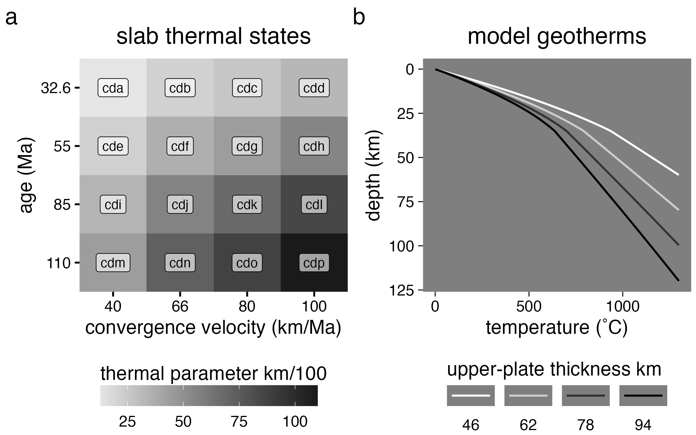
Figure 2.2: Range of thermo-kinematic boundary conditions used in numerical experiments. (a) Thermal parameters (grayscale) range from 13 to 110 km/100 and broadly reflect the distribution of oceanic plate ages and convergence velocities in modern subduction zones. Model names include the prefix “cd” for “coupling depth” with increasing alphabetic suffixes. Note that neither axes are continuous. (b) Upper-plate thickness (\(Z_{UP}\)) is defined by a range of continental geotherms. Geotherms were constructed using a one-dimensional steady-state conductive cooling model with T(z=0) = 0 ˚C, \(\vec{q}\)(z=0) = 59, 63, 69, 79 mW/m\(^2\), and constant radiogenic heating of 1.0 \(\mu\)W/m\(^3\) for a 35 km-thick crust and 0.022 \(\mu\)W/m\(^3\) for the mantle. Continental geotherms are calculated up to 1300 ˚C with a constant 0.5 ˚C/km gradient (the mantle adiabat) extending to the base of the model domain.

Table 2.1: Material properties used in numerical experiments

Material	\(\rho\)	\(H_2O\)	Flow Law	\(log_{10}A\)	\(E\)	\(V\)	\(n\)	\(\phi\)	\(\sigma_{crit}\)	\(k_1\)	\(k_2\)	\(k_3\)	\(H\)
	\(kg/m^3\)	\(wt.\%\)			\(kJ/mol\)	\(J/MPa\cdot mol\)			\(MPa\)				\(\mu W/m^3\)
sediments	2600	5.0	wet quartzite	-3.5	154.0	3.0	2.3	0.15	0.03	0.64	807	4e-06	2.000
felsic crust	2700		wet quartzite	-3.5	154.0	3.0	2.3	0.45	0.03	0.64	807	4e-06	1.000
basalt	3000	5.0	plag an75	-3.5	238.0	8.0	3.2	0.45	0.03	1.18	474	4e-06	0.250
gabbro	3000		plag an75	-3.5	238.0	8.0	3.2	0.45	0.03	1.18	474	4e-06	0.250
mantle dry	3300		dry olivine	4.4	540.0	20.0	3.5	0.45	0.30	0.73	1293	4e-06	0.022
mantle hydrated	3300	0.5	wet olivine	3.3	430.0	10.0	3.0	0.45	0.24	0.73	1293	4e-06	0.022
serpentine	3200	2.0	serpentine	3.3	8.9	3.2	3.8	0.15	3.00	0.73	1293	4e-06	0.022
key: \(A\): material constant, \(E\), \(V\): activation energy and volume, \(n\): power law exponent, \(\phi\): internal friction angle, \(\sigma_{crit}\): critical stress, \(k_1\)-\(k_3\): thermal conductivity constants, \(H\): heat production
constants: \(C_p\): heat capacity = 1 [kJ/kg], \(\alpha\): expansivity = 2\(\times 10^{-5}\) [1/K], \(\beta\): compressibility = 0.045 [1/MPa]
thermal conductivity: \(k\) [W/mK] = \((k_1+\frac{k_2}{T+77})\times exp(k_3 \cdot P)\) with \(P\) in [MPa] and \(T\) in [K]
references: Turcotte & Schubert (2002), Ranalli (1995), Hilairet et al. (2007), Karato & Wu (1993)

2.2.1 Initial Setup and Boundary Conditions

Simulations are 2000 km wide and 300 km deep (Figure 2.1). In the model domain, three governing equations of heat transport, momentum, and continuity are discretized and solved with a conservative finite-difference marker-in-cell approach on a fully staggered grid as outlined in Gerya & Yuen (2003). Numerical resolution is nonuniform with higher resolution (1 \(\times\) 1 km) in a 600 km wide area surrounding the contact between the oceanic plate and continental margin, then gradually changing to lower resolution towards the model boundaries (5 \(\times\) 1 km, x- and z-directions, respectively). The left and right boundaries are free-slip and thermally insulating (Figure 2.1a, b). Implementation of “sticky” air and water allows for a free topographical surface with a simple linear sedimentation and erosion model. The lower boundary is open to allow for oceanic plate descent with a spontaneous subduction angle (Burg & Gerya, 2005).

A horizontal convergence force is applied to both plates in a rectangular region far from the continental margin (Figure 2.1c). An initial weak layer cutting the lithosphere permits subduction to initiate. The high-viscosity (\(\eta = 10^{25}\) Pa \(\cdot\) s) rectangular convergence regions apply constant horizontal velocities without deforming the lithosphere. Subduction angle is governed by free-motion of the subducting plate. Similarly, subduction velocity varies with time in response to extension or shortening of the overriding plate. \(\Phi\) is thus calculated as the product of the horizontal convergence velocity and the oceanic plate age (cf. Kirby et al., 1991; McKenzie, 1969). For convenience and consistency with the literature, this study presents \(\Phi\) in units of km/100 (Figure 2.2a).

2.2.2 Rheologic Model

Contributions from dislocation and diffusion creep are accounted for by computing a composite rheology for ductile rocks, \(\eta_{eff}\): \[\begin{equation} \begin{aligned} \frac{1}{\eta_{eff}} = \frac{1}{\eta_{diff}} + \frac{1}{\eta_{disl}} \end{aligned} \tag{2.1} \end{equation}\] where \(\eta_{diff}\) and \(\eta_{disl}\) are effective viscosities for diffusion and dislocation creep.

For the crust and serpentinized mantle, \(\eta_{diff}\) and \(\eta_{disl}\) are computed as: \[\begin{equation} \begin{aligned} \eta_{diff} &= \frac{1}{2} \ A \ \sigma_{crit}^{1-n} \ \exp\left[\frac{E+PV}{RT}\right] \\ \eta_{disl} &= \frac{1}{2} \ A^{1/n} \ \dot{\varepsilon}_{II}^{(1-n)/n} \ \exp\left[\frac{E+PV}{nRT}\right] \end{aligned} \tag{2.2} \end{equation}\] where \(R\) is the gas constant, \(P\) is pressure, \(T\) is temperature in \(K\), \({\dot{\varepsilon}}_{II} = \sqrt{\frac{1}{2}{{\dot{\varepsilon}}_{ij}}^{2}}\) is the square root of the second invariant of the strain rate tensor, \(\sigma_{crit}\) is an assumed diffusion-dislocation transition stress, and \(A\), \(E\), \(V\) and \(n\) are the material constant, activation energy, activation volume, and stress exponent, respectively (Table 2.1, Hilairet et al., 2007; Ranalli, 1995).

For the mantle, \(\eta_{diff}\) and \(\eta_{disl}\) are computed as (Karato & Wu, 1993): \[\begin{equation} \begin{aligned} \eta_{diff} &= \frac{1}{2} \ A^{-1} \ G \ \left[\frac{h}{b}\right]^{m/n} \ \exp\left[\frac{E+PV}{RT}\right] \\ \eta_{disl} &= \frac{1}{2} \ A^{-1/n} \ G \ \dot{\varepsilon}_{II}^{(1-n)/n} \ \exp\left[\frac{E+PV}{nRT}\right] \end{aligned} \tag{2.3} \end{equation}\] where \(b\) = 5 \(\times\) 10\(^{-10}\) m is the Burgers vector, \(G\) = 8 \(\times\) 10\(^{10}\) Pa is shear modulus, \(h\) = 1 \(\times\) 10\(^{-3}\) m is the assumed grain size, \(m\) = 2.5 is the grain size exponent, and the other flow law parameters are given in Table 2.1. Viscosity is limited in all numerical experiments from \(\eta_{min}\) = 10\(^{17}\) Pa \(\cdot\) s to \(\eta_{max}\) = 10\(^{25}\) Pa \(\cdot\) s.

An effective visco-plastic rheology is achieved by limiting \(\eta_{eff}\) with a brittle (plastic) yield criterion: \[\begin{equation} \eta_{eff} \leq \frac{C + \phi \ P}{2 \ \dot{\varepsilon}_{II}} \tag{2.4} \end{equation}\] where \(\phi\) is the internal friction coefficient, \(C\) cohesive strength at \(P\) = 0, and \({\dot{\varepsilon}}_{ij}\) is the strain rate tensor (Table 2.1).

2.2.3 Defining Geotherms and Lithospheric Thickness

Oceanic crust is modelled as 1 km of sediment cover overlying 2 km of basalt and 5 km of gabbro (Figure 2.1a). Oceanic lithosphere is continually made at a pseudo-mid-ocean ridge at the left boundary of the model (Figure 2.1b). An enhanced vertical cooling condition applied at 200 km from left boundary adjusts for the proper oceanic plate age, and therefore its lithospheric thickness as it enters the trench (Agrusta et al., 2013). Oceanic plate ages range from 32.6 to 110 Ma and convergence velocities from 40 to 100 km/Ma (Figure 2.2a). This range of parameters broadly reflects the middle-range of modern global subduction systems (Syracuse & Abers, 2006).

Initial continental geotherms are determined by solving the heat flow equation in one-dimension to 1300 ˚C (Figure 2.2b). This study assumes a fixed temperature of 0 ˚C at the surface, constant radiogenic heating of 1 \(\mu\)W/m\(^3\) in the 35 km-thick continental crust, 0.022 \(\mu\)W/m\(^3\) in the mantle, with thermal conductivities of 2.3 W/mK and 3.0 W/mK for the continental crust and mantle, respectively. Above, 1300 ˚C, temperature is assumed to constantly increase by 0.5 ˚C/km (the mantle adiabat) to the base of the model domain.

Many studies define the base of the continental lithosphere at the 1300 ˚C isotherm, but it can be determined directly by visualizing viscosity and strain rate as the model progresses. The mechanical base of the lithosphere (\(Z_{UP}\)) in the models generally occurs near the 1100 ˚C isotherm—characterized by a rapid decrease in viscosity and increase in strain rate (Figures A.2, A.3, A.4). As such, this study considers oceanic and continental lithospheres as mechanical layers defined by viscosity, rather than defined merely by temperature. \(Z_{UP}\) corresponding to backarc surface heat flow of 59, 63, 69, and 79 mW/m\(^2\) are used in this study (Figure 2.2b).

2.2.4 Metamorphic (De)hydration Reactions

Using Lagrangian markers (Harlow, 1962, 1964) to store and update material properties and PT-strain fields allows for straight-forward numerical implementation of metamorphic reactions. This approach is key to regulating mechanical coupling dynamically in subduction zone simulations. For example, dehydration (eclogitization) of the oceanic plate and (de)stabilization of serpentine in the upper-plate mantle may be effectively modelled by tracing marker PT-time paths while changing marker properties according to thermodynamically-stable mineral assemblages (e.g. Connolly, 2005). For computational efficiency, however, water contents in this study are not computed by iteratively solving thermodynamic systems of equations.

Instead, gradual eclogitization of oceanic crust is computed as a linear function of lithostatic pressure to a maximum depth of 150 km, or temperature of 1427 ˚C, while including garnet-in and plagioclase-out reactions defined by Ito & Kennedy (1971). Mantle (de)hydration is computed according reactions boundaries defined by Schmidt & Poli (1998) with a maximum water content of 2 \(wt.\%\) (explained below). This approach effectively simulates continuous influx of water to the upper-plate mantle with relatively low computational cost, beginning with compaction and release of connate water at shallow depths, followed by a sequence of reactions consuming major hydrous phases (chlorite, lawsonite, zoisite, chloritoid, talc, amphibole, and phengite) in different parts of the hydrated basaltic crust (Schmidt & Poli, 1998; van Keken et al., 2011).

The extent of metamorphic reaction effects on mechanical coupling, and the exact (de)hydration reaction(s) likely responsible, are unknown. However, formation of brucite and serpentine from dry olivine near the plate interface are inferred to strongly regulate mechanical behavior (Agard et al., 2016; Hyndman & Peacock, 2003; Peacock & Hyndman, 1999). Brucite notably breaks down at much lower temperatures than serpentine (Schmidt & Poli, 1998), so serpentine (de)stabilization arguably represents the key transition from a weak-to-strong upper-plate mantle deep in subduction zones. This study elects an implementation of serpentine (de)hydration for this reason. The reaction is assumed to be abrupt and discontinuous, which is a fine approximation for near-endmember compositions like (Mg-rich) peridotites. The PT conditions of the reaction \(antigorite \Leftrightarrow olivine + orthopyroxene + H_{2}O\) were numerically implemented by the following equation (after Schmidt & Poli, 1998): \[\begin{equation} T_{atg-out}(z)= \begin{cases} 751.50+6.008\times10^{-3}z-3.469\times10^{-8}z^2,& \text{for } z < 63000m \\ 1013.2-6.039\times10^{-5}z-4.289\times10{-9}z^2,& \text{for } z>63000m \end{cases} \tag{2.5} \end{equation}\] where \(z\) is the depth of a marker from the surface in meters and \(T\) is temperature in Kelvins. This reaction boundary is consistent to within 25 ˚C of more recent experiments by Shen et al. (2015). Markers with internal temperature exceeding \(T_{atg-out}(z)\) spontaneously form \(olivine + orthopyroxene + H_{2}O\) and release their crystal-bound water. This implementation tacitly assumes thermodynamic equilibrium and is common to many versions of I2VIS.

Oceanic plates of different ages are also tacitly assumed to dehydrate similarly with the above implementation. However, older (colder) oceanic plates are expected to carry water to greater depths than younger (warmer) plates because of relatively delayed water-releasing reactions (Peacock, 1996). Abrupt water release with serpentine dehydration (Equation (2.5)) was tested to model deep water retention in cold oceanic plates. Mechanical coupling behavior was indistinguishable from gradual water release models. This implies rates of water release are less important than the depth of serpentine stability. Explicitly modelling other major dehydration reactions are thus unlikely to significantly affect mechanical coupling behavior, yet likely to introduce numerical artifacts at great computational cost. A simplified gradual water release model for all oceanic plates is therefore preferred.

Water released by rock forms discrete fluid particles that migrate with relative velocities defined by local deviatoric (non-lithostatic) pressure gradients (see Appendix A.3, Faccenda et al., 2009). Fluid velocities are scaled by a 10 cm/yr vertical percolation velocity to account for purely lithostatic pressure gradients in the mantle (Gorczyk et al., 2007). Fluid particles migrate until encountering rock that can consume additional water by equilibrium hydration or melting reactions, (Equation A.4).

The shallow upper-plate mantle can theoretically store large amounts of water as serpentine may contain up to 13 \(wt.\%\) water (Reynard, 2013) and is generally stable at shallow mantle conditions. Thermodynamic models predict 8 \(wt.\%\) water in the shallow upper-plate mantle (Connolly, 2005). However, seismic studies suggest most shallow upper-plate mantles are only partially serpentinized (< 20-40%), equating to water contents of approximately 3-6 \(wt.\%\) (Abers et al., 2017; Carlson & Miller, 2003). Many modes of mantle hydration are documented or inferred, including evidence for channelized fluid flow within ophiolites exhumed from subduction zones (Angiboust et al., 2012a, 2014a; Plümper et al., 2017; Zack & John, 2007). This study limits mantle wedge hydration to \(\leq\) 2 \(wt.\%~H_{2}O\) and assumes any excess \(H_{2}O\) exits the system through channelized fluid flow during plastic or brittle deformation (Davies, 1999b).

2.2.5 Visualization and Determination of Coupling Depth

The rheologic model and thermo-kinematic boundary conditions described in the previous sections always results in plate motions towards the left boundary (slab-rollback). Relatively high dip angles and extreme subduction velocities in some high-\(\Phi\) experiments cause chaotic behavior by 10 Ma as the upper-plate is stretched thin and mechanical interference occurs between trench sediments and the high-viscosity convergence region 200 km from the left boundary. Numerical solutions are stable for most experiments, however, reaching quasi-steady state by 5 Ma. An additional 5 Ma is allowed to ensure stable geodynamics before observing coupling depth. Surface heat flow, rock type, temperature, viscosity, strain rate, shear heating, and velocity fields are visualized at approximately 10 Ma (e.g. Figure 2.3) for all 64 experiments to assess geodynamics and solution stability (Figure A.1).

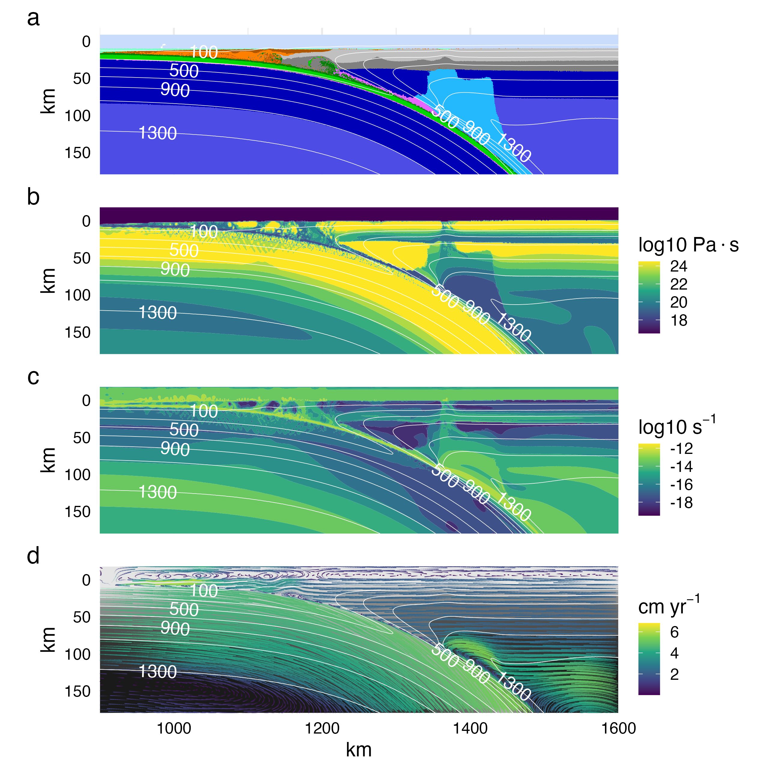
Figure 2.3: Visualizing model cdf with a 78 km upper-plate lithosphere at approximately 10 Ma. (a) Rock type shows a thin serpentine layer (pink) lubricating the plate interface. Note that low melt volumes are inconspicuous and quickly extracted. (b) Viscosity shows high contrast between the oceanic plate and serpentinized upper-plate mantle at shallow levels. Viscosity contrast disappears where serpentine becomes unstable. (c) Streamlines show focused mantle flow towards the interface, coinciding with the lower limit of serpentine stability. Note the converging isotherms that imply a feedback between heat transfer, serpentine destabilization, and mechanical coupling. (d) Strain rate shows localized deformation in the serpentine layer along the plate interface. Note that deformation in the upper-plate mantle is restricted to viscous flow beneath the lithosphere and along narrow, subvertical melt conduits. Rock type colors are the same as Figure 2.1.

After approximately 10 Ma of subduction coupling depth is determined directly from viscosity by finding the approximate area where strength contrasts between serpentinized- and non-serpentinized upper-plate mantle diminishes to < 10\(^2\) Pa \(\cdot\) s. The node nearest to this region is assigned as the coupling depth. This study assumes mechanical coupling occurs instantaneously and at a single node. Mechanical coupling in reality must be dispersed across a finite length along the plate interface, however. At the numerical resolution the experiments, coupling-like viscosity contrasts are similar within a small area (approximately 5 \(\times\) 5 km or 5 \(\times\) 5 nodes), giving a qualitative uncertainty coupling depth on the order of 2.5 km.

2.3 Results

2.3.1 Coupling Depth Estimators

Coupling depth (\(Z_{cpl}\)) correlates strongly with upper-plate thickness (\(Z_{UP}\)) and weakly with \(\Phi\) across all 64 numerical models (Table A.3, Figures A.6 & A.7). The responsiveness of coupling depth to \(Z_{UP}\) but not to \(\Phi\) is a key result of this study. The following equation minimizes standard least squares while optimizing the number of parameters, p value, and \(R^2\) for all possible permutations of the variables \(Z_{UP}\) and \(\Phi\) in linear and quadratic forms: \[\begin{equation} Z_{cpl} = 4.95\times 10^{-3}\ Z_{UP}^{2}\ -\ 9.27\times 10^{-2}\ \Phi\ +\ 63.6 \tag{2.6} \end{equation}\] where \(Z_{cpl}\) is coupling depth in km and \(\Phi\) is the thermal parameter in km/100. Regression summaries show both linear and quadratic models of \(Z_{cpl}\) vs. \(Z_{UP}\) and \(\Phi\) fit experimental results well (Tables A.1 & A.2). Equation (2.6) represents a statistical model formulated with observations from physics-based simulations of subduction. Equation (2.6) is useful for estimating coupling depths in active subduction zones where \(\Phi\) is known and \(Z_{UP}\) can be inverted from surface heat flow.

Sensitivity of coupling depth to upper-plate thickness and \(\Phi\) is apparent when visualizing Equation (2.6) and other regression models across \(Z_{UP}\) and \(\Phi\) space 2.4. Applying Equation (2.6) to 17 active subduction zone segments (Table 2.2) gives a wide range of estimated coupling depths, similar to the numerical simulations in this study. The distribution of estimated coupling depths, however, is relatively narrow and quasi-normal, with a mean of \(\sim\) 82 km and standard deviation of 7 km (Figure 2.4d).

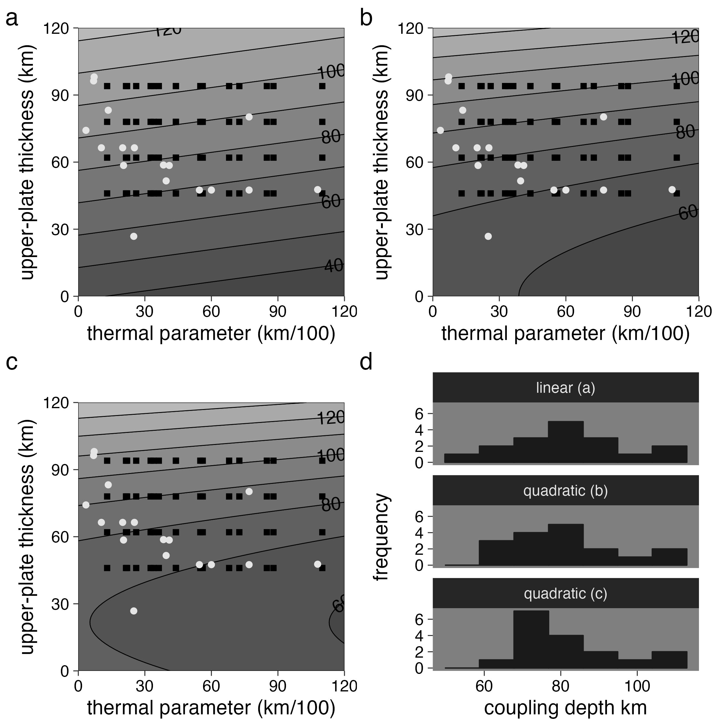
Figure 2.4: Multivariate regressions and estimated coupling depth (\(Z_{cpl}\)) for 17 active subduction zone segments. Contoured plots show estimated \(Z_{cpl}\) (contours) as a function of thermal parameter (\(\Phi\)) and upper-plate thickness (\(Z_{UP}\)) for linear (a) and quadratic (b, c) regressions. The best fit regression is panel b (Equation (2.6), see Tables A.1 and A.2). Black squares are numerical experiments used to fit the contours. White points represent active subduction zones (Table 2.2). Contours imply \(Z_{cpl}\) depends strongly on \(Z_{UP}\). While some estimated \(Z_{cpl}\) for subduction zones with similar \(\Phi\) are quite different (e.g. Alaska vs. N. Sumatra), some estimated \(Z_{cpl}\) are quite similar for subduction zones with very different \(\Phi\) (e.g. Kamchatka vs. N. Cascadia). (d) Distributions of estimated \(Z_{cpl}\) for 17 active subduction zones shown in (a), (b), and (c). These 17 segments span a large range of \(\Phi\) but are expected to have a relatively narrow distribution of \(Z_{cpl}\) (82 ± 14 km) according to the regressions in (a), (b), and (c).

Table 2.2: Estimated coupling depths for active subduction zones

Segment	\(\vec{q}\)	\(Z_{UP}\)	\(\Phi\)	\(Z_{cpl}^a\)	\(Z_{cpl}^b\)	\(Z_{cpl}^c\)
	mW/m\(^2\)	km	km/100	km	km	km
N. Cascadia	75	74.2	3.4	92	91	90
Nankai	69	96.3	6.9	107	109	110
Mexico	72	98.1	7.2	108	111	112
Columbia-Ecuador	80	66.4	10.4	86	84	84
S.C. Chile	80	66.4	20.0	85	84	83
Kyushu	69	83.2	13.5	97	97	96
N. Sumatra	120	26.8	25.0	57	65	68
Alaska	80	66.4	25.3	85	83	82
N. Chile	85	58.7	38.4	78	77	77
N. Costa Rica	80	58.5	20.4	80	79	78
Aleutians	75	51.6	39.6	73	73	73
N. Hikurangi	80	58.5	41.0	78	77	76
Mariana	80	47.5	54.6	69	70	70
Kermadec	80	47.5	60.0	68	69	70
Kamchatka	70	80.2	77.0	89	88	88
Izu	80	47.5	77.0	67	68	68
NE Japan	88	47.7	107.9	64	65	65
estimators: a: \(Z_{cpl}=Z_{UP}+\Phi\), b: \(Z_{cpl}=Z_{UP}^2+\Phi\), c: \(Z_{cpl}=Z_{UP}+Z_{UP}^2+\Phi\)
references: Currie & Hyndman (2006), Wada & Wang (2009)

2.3.2 Surface Heat Flow

Upper-plate surface heat flow remains relatively stable and reflects initial upper-plate geotherms in the backarc region for experiments with low to moderate \(\Phi\) (Figure A.5). However, high-amplitude and high-frequency positive surface heat flow deviations in the upper-plate are common in all experiments, especially for high-\(\Phi\) experiments. These deviations correspond to extensional deformation and heat transport via lithospheric thinning and melt migration. These features are apparent as subvertical low viscosity, high strain rate columns originating from the plate interface (Figure 2.3b, d) and point to potential sources of error when inverting surface heat flow in active subduction zones. Notably, the backarc is relatively unaffected by fluid and melt migration compared to the forearc. Estimating upper-plate thickness by inverting surface heat flow in the backarc is therefore preferable to forearc surface heat flow.

Surface heat flow across all numerical experiments is similar in the forearc region (normalized distance \(\leq\) 0.75, Figure 2.5). In contrast, surface heat flow extending behind the arc region (normalized distance > 0.75, Figure 2.5) increases systematically, then levels off at values reflecting initial continental geotherms (i.e. reflecting initial upper-plate thickness). In reality, surface heat flow depend on fault slip rates and rates of volcanic outputs. However, heat flow in the behind the arc may remain in steady-state if rates of volcanism and crustal thinning by extension are low (Currie et al., 2004; Currie & Hyndman, 2006).

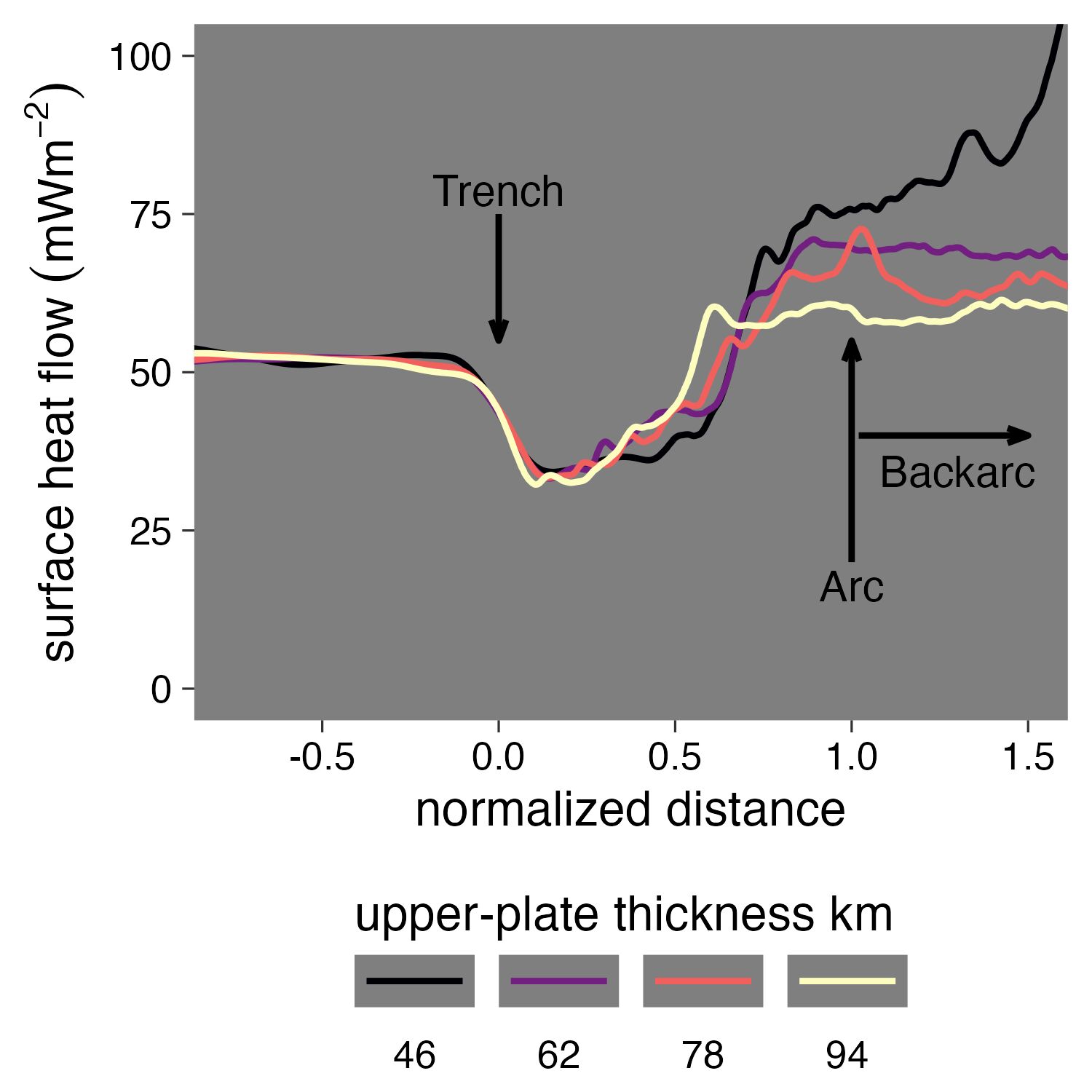
Figure 2.5: Surface heat flow (\(\vec{q}\)) vs. normalized distance for model cdf with upper-plate thickness (\(Z_{UP}\)) ranging from 46 to 94 km. The distribution of \(\vec{q}\) in the forearc (normalized distance between 0.0 and 1.0) is narrow and shows little variance until near the arc (normalized distance between 0.75 and 1.0). The broad distribution of \(\vec{q}\) behind the arc (normalized distance > 1.0) reflects the broad distribution of initial continental geotherms (\(Z_{UP}\)). Any simple relationship between \(\vec{q}\) and \(Z_{UP}\) may be obscured by heating from extension or vertical migration of fluids, especially within the arc-region (high-amplitude fluctuations).

2.4 Discussion

2.4.1 Dynamic Feedbacks Regulating Plate Coupling

A clear association between plate coupling and the reaction \(antigorite \Leftrightarrow olivine + orthopyroxene + H_{2}O\) is observed in all experiments. A relatively narrow serpentine channel quickly forms above the dehydrating oceanic plate, localizing strain, lubricating the plate interface, and inhibiting transfer of shear stress between plates (e.g. Agard et al., 2016; Ruh et al., 2015). This mechanical behavior is a direct consequence of a sharp rheologic change dependent on the location of serpentine dehydration reaction described in Section 2.2.4 and its effect on the rheologic model described in Section 2.2.2. Interactions among viscosity changes, serpentine dehydration, and heat transfer are regulated by competing dynamic feedbacks acting in the upper-plate. In summary, cooling and hydration of the shallow upper-plate mantle (serpentine stabilization) and heating from circulating asthenospheric mantle beneath the upper-plate lithosphere (driven by mechanical coupling) compete to stabilize coupling depth (Figure 2.6).

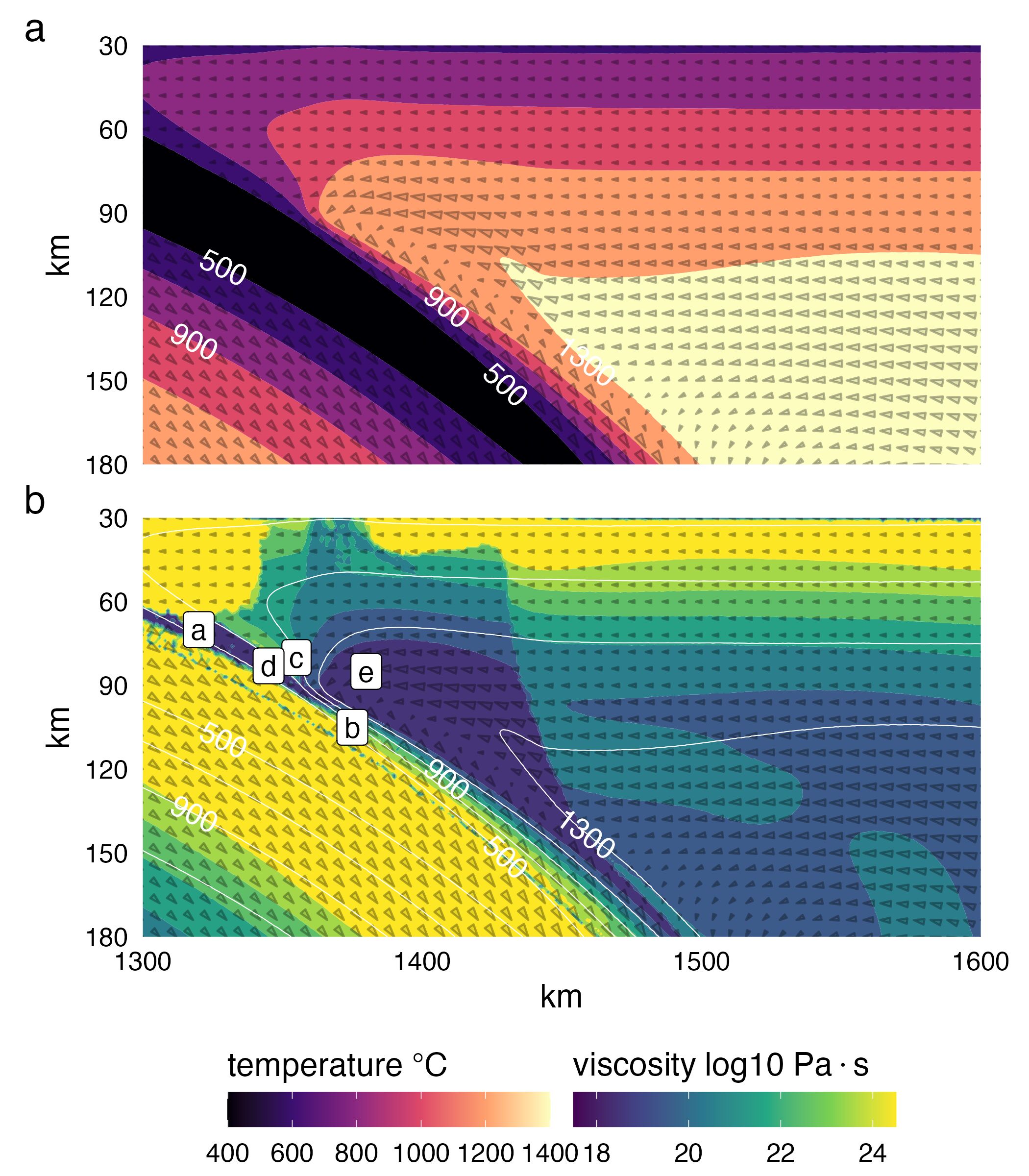
Figure 2.6: Visualizing viscosity and mantle flow near the coupling region at approximately 10 Ma for model cdf with upper-plate thickness of 78 km. (a) Temperature field. (b) Strong mantle flow beneath the lithospheric base (1100˚C) transfers heat towards the coupling region. Viscosity indicates coupling at the point where the viscosity contrast between the slab and mantle approaches zero (between points b & d). Reference points a-e are used for discussing coupling dynamics and thermal feedbacks (see Section 2.4.2).

The entire process can be conceptualized with Figure 2.6 as follows. The upper-plate mantle cools via diffusive heat loss to the oceanic plate along the entire length of the plate interface (Figure 2.6a). At shallow depths, water released from the oceanic plate stabilizes serpentine in the overriding upper-plate mantle, effectively decoupling the two plates (Figure 2.6b, point a). A positive feedback stabilizes serpentine to greater depths as decoupled plates stagnate the upper-plate mantle, promoting further cooling and formation of serpentine. Numerical experiments imply only a thin layer of serpentine is sufficient to trigger this feedback.

Deeper along the plate interface, beyond the stability of serpentine, diffusive heat loss from the upper-plate mantle to the slab forms a thickening layer of high-viscosity mantle atop the oceanic plate (Figure 2.6b, point b). Downward motion of the oceanic plate, plus accreted high-viscosity mantle (Figure 2.6b, point b) relative to the deepest extent of the stiff upper-plate mantle (Figure 2.6b, point c) creates a pressure gradient that attracts flow of the weakest materials—serpentine from the up-dip direction (Figure 2.6b, point d)—and hot mantle from below (Figure 2.6b, point e). Flow of hot mantle into the necking region between points b and c in Figure 2.6 is analogous to passive asthenospheric upwelling toward a mid-ocean ridge where two strong cooling lithospheric plates diverge. Highly efficient heat advection from the warm upper-plate asthenospheric mantle (Figure 2.6a) prevents formation of sperentine—thus regulating and stabilizing the coupling depth.

Coupling mechanics apparent from numerical experiments can be described in terms of competing positive and negative feedbacks. The positive feedback involves addition of water into a diffusively cooling, shallow mantle to produce serpentine. The negative feedback involves serpentine destabilization by advection of heat from the deeper upper-plate asthenospheric mantle. Such thermal-petrologic-mechanical feedbacks drive coupling depth towards steady-state. The numerical experiments in this study imply a finely-tuned balance of serpentine stability can maintain coupling depths in subduction zones for potentially 10’s of Ma.

2.4.2 Coupling Responses to \(Z_{UP}\) and \(\Phi\)

How does upper-plate thickness influence coupling depth? Numerical experiments point to the upper-plate lithosphere-asthenosphere boundary as an important feature constraining coupling mechanics as it defines the permissible flow field in the upper-plate (Figure 2.7a-d). Thin upper-plate lithospheres (Figure 2.7a, b) permit shallow mantle flow and advection of heat farther up the plate interface. Thin upper-plate lithospheres thereby raise coupling depths by raising serpentine stability up the plate interface. Thick upper-plate lithospheres (Figure 2.7c, d) restrict mantle wedge flow to deeper levels, deepening serpentine stability and mechanical coupling.

The thermal state of the slab, as represented by \(\Phi\), has almost no effect on coupling depth by comparison. Relative insensitivity of coupling depth to \(\Phi\) is consistent with previous studies of active subduction zones (Furukawa, 1993; Wada & Wang, 2009). The irresponsiveness of coupling depth to changes in \(\Phi\) is perhaps due to competing cooling and heating effects driven by the subducting oceanic plate. For example, high-\(\Phi\) oceanic plates (older plates with higher velocities) cool the upper-plate mantle more effectively, but also effectively heat the interface by driving stronger mantle circulation. In contrast, low-\(\Phi\) oceanic plates (younger plates with lower velocities) are less effective in cooling the upper-plate mantle, but also ineffectively heat the interface by ineffectively driving mantle circulation. That is, the shallow vs. deep dynamic effects of \(\Phi\) tend to cancel each other, explaining the lack of correlation between coupling depth and \(\Phi\).

2.4.3 Estimating Coupling Depths in Subduction Zones

Theoretically, coupling depth can be estimated directly by fitting forearc surface heat flow data using forward modelling approaches (e.g. Wada & Wang, 2009). However, forward approaches typically adjust coupling depth independently from upper-plate thickness, which is inconsistent with an inherent link between coupling depth and upper-plate thickness discussed in Section 2.4 (e.g. Figures 2.5 & 2.7). Moreover, many additional heat sources (e.g. shear heating and crustal plutonism, Gao & Wang, 2014; Rees Jones et al., 2018) may contribute to forearc surface heat flow—increasing uncertainty when inverting upper-plate thickness from surface heat flow.

Assuming low degrees of backarc extension, estimating coupling depth in active subduction zones using Equation (2.6) with \(Z_{UP}\) inverted from backarc surface heat flow is preferable to avoid additional uncertainties stemming from seismic and volcanic activity in the forearc. However, while \(\Phi\) is inventoried for most active subduction zones (Syracuse & Abers, 2006), a corresponding dataset of \(Z_{UP}\) does not exist. Several geophysical and petrologic methods might be considered for independent estimates of \(Z_{UP}\) (e.g. seismic velocities, flexure, heat flow, mantle xenoliths). Backarc surface heat flow is still a good choice, however, because of its direct correspondence with \(Z_{UP}\). For example, \(Z_{UP}\) may be estimated using simple one-dimensional heat transport models assuming values for radiogenic heat production in the crust (Rudnick et al., 1998). Special attention must be paid to crustal processes, including extension and magmatism, because additional heating will underestimate \(Z_{UP}\) and, consequently, underestimate coupling depth.

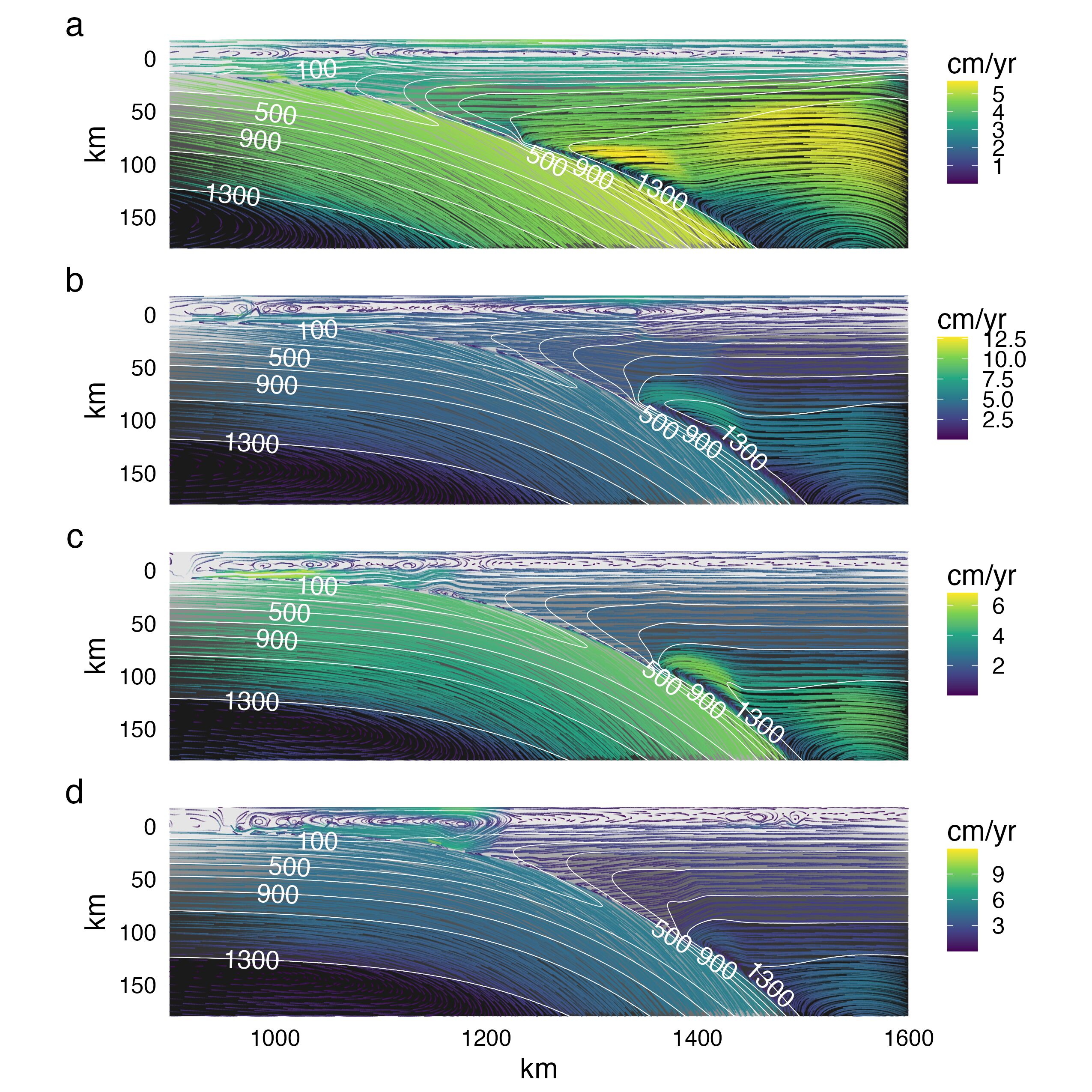
Figure 2.7: Visualizing mantle flow at approximately 10 Ma for model cdf with upper-plate thickness of (a) 46, (b) 62, (c) 78, and (d) 94 km. All experiments are plotted on the same scale and location within the model domain. The flow of warm mantle is restricted to below the 1100˚C isotherm, which corresponds to the base of the upper-plate lithosphere (\(Z_{UP}\)). A minimum coupling depth (\(Z_{cpl}\)) appears to exist as models with extremely thin lithospheres (a) exhibit coupling at \(\sim\) 70-80 km depth. \(Z_{cpl}\) generally increases with increasing \(Z_{UP}\) as mantle flow and advective heat transport are restricted to greater depths.

2.4.4 Globally Similar Coupling Depths?

A \(Z_{cpl}\) distribution of 82 ± 14 km (2\(\sigma\)) estimated for active subduction zones in this study (Figure 2.4d) roughly match the preferred \(Z_{cpl}\) inferred from forearc surface heat flow for Cascadia and NE Japan (75-80 km, Syracuse et al., 2010; Wada & Wang, 2009) km. The range of \(Z_{cpl}\) estimated for active subduction zones in this study (Figure 2.4d) is relatively broad, however. For example, omitting Mexico and Nankai because their \(\Phi\) values fall outside the range of \(\Phi\) used for numerical experiments, estimated coupling depths range from almost 100 km (Kyushu) to approximately 65 km (Sumatra and NE Japan, Table 2.2).

Coupling depth in active subduction zones are commonly assumed to be narrowly distributed around 70-80 km (Syracuse et al., 2010; Wada & Wang, 2009). The strong correlation between \(Z_{UP}\) and \(Z_{cpl}\) found from numerical experiments imply uniform coupling depths are possible if upper-plate thickness are globally uniform. The surface heat flow dataset compiled by Wada & Wang (2009) (Table 2.2) shows average backarc surface heat flow are indeed similar among active subduction zones—implying a narrow distribution of coupling depths (Figure 2.4d). Much of their dataset is based on Currie & Hyndman (2006), who estimate upper-plate thickness for 10 circum-Pacific subduction zones of 50-60 km (defined by the 1200 ˚C isotherm). Uniformly thin upper-plate thickness are corroborated by uniformly high heat flow (> 70 mW/m\(^2\)), thermobarometric constraints on mantle xenoliths, and P-wave velocities (Currie & Hyndman, 2006). An attempt is made to further corroborate the uniformity of upper-plate thickness in Chapter 3 by interpolating surface heat flow near active subduction zones.

Although it still curious why upper-plates among subduction zones may have similar thicknesses, one can assume it is likely related to some processes of lithospheric erosion proposed for subarc lithosphere. These include: lithospheric delamination induced by lower crust eclogitization (Sobolev & Babeyko, 2005), small-scale convection caused by hydration-induced mantle wedge weakening (Arcay et al., 2006), thermal erosion (England & Katz, 2010), mechanical weakening by percolating melts (Gerya & Meilick, 2011), and subarc foundering of magmatic cumulates (Jull & Kelemen, 2001). Most of these mechanisms are thus strongly related to mantle wedge hydration, melting, and melt transport toward volcanic arcs.

The metamorphic rock record may also imply consistency among coupling depths in subduction zones. For example, the demise of a serpentine channel and onset of coupling may provide a natural barrier such that rocks are more likely to be exhumed from within the channel than from below it. The relative abundance of blueschists and eclogites should then be greater for pressures below estimated coupling depths (approximately 2.4 GPa or 70-80 km) than above them.

2.5 Conclusions

Three important results are highlighted in this study:

1. Coupling depth is stabilized near the base of the upper-plate lithosphere by competing dynamic feedbacks regulating heat transport, serpentine dehydration, and mechanical coupling in the upper-plate mantle.

2. A simple expression fitted to coupling depths observed in numerical experiments allows the coupling depths to be estimated for active subduction zones by inverting upper-plate thickness from surface heat flow.

3. Uniform surface heat flow in circum-Pacific subduction zones (Currie & Hyndman, 2006; Wada & Wang, 2009) may indicate uniform coupling depths at approximately 80 km.

Questions remain, however, including: how do warm (thin) upper-plates persist over 100’s of kilometers behind arcs and throughout the lifespan of subduction zones? How abruptly are dehydration reaction occurring along the subduction interface? How can expressions like Equation (2.6) be improved using natural datasets? Each of these questions may be considered for future research.

3 A Comparison of Surface Heat Flow Interpolations Near Subduction Zones

Abstract

The magnitude and spatial extent of heat fluxing through the Earth’s surface depend on the integrated thermal state of Earth’s lithosphere (conductive heat loss) plus heat generation (e.g. from seismic cycles and radioactive decay) and heat transfer via advection (e.g. by fluids, melts, and plate motions). Surface heat flow observations are thus critically important for understanding the thermo-mechanical evolution of subduction zones. Yet evaluating regional surface heat flow patterns across tectonic features remains difficult due to sparse observations irregularly-spaced at distances from 10\(^{-1}\) to 10\(^3\) km. Simple sampling methods (e.g. 1D trench-perpendicular transects across subduction zones) can provide excellent location-specific information but are insufficient for evaluating lateral (along-strike) variability. Robust interpolation methods are therefore required. This study compares two interpolation methods based on fundamentally different principles, Similarity and Kriging, to (1) investigate the spatial variability of surface heat flow near 13 presently active subduction zone segments and (2) provide insights into the reliability of such methods for subduction zone research. Similarity and Kriging predictions show diverse surface heat flow distributions and profiles among subduction zone segments and broad systematic changes along strike. Median upper-plate surface heat flow varies 25.4 mW/m\(^2\) for Similarity and 42.4 mW/m\(^2\) for Kriging within segments, on average, and up to 40.7 mW/m\(^2\) for Similarity and up to 90.5 mW/m\(^2\) for Kriging among segments. Diverse distributions and profiles within and among subduction zone segments imply spatial heterogeneities in lithospheric thickness, subsurface geodynamics, or near-surface perturbations, and/or undersampling relative to the scale and magnitude of spatial variability. Average accuracy rates of Similarity (28.8 mW/m\(^2\)) and Kriging (32.2 mW/m\(^2\)) predictions are comparable among subduction zone segments, implying either method is viable for subduction zone research. Importantly, anomalies and methodological idiosyncrasies identified by comparing Similarity and Kriging can aid in developing more accurate regional surface heat flow interpolations and identifying future survey targets.

3.1 Introduction

The amount of heat escaping Earth’s surface depends on the integrated thermal state of Earth’s lithosphere, plus heat-transferring and heat-generating subsurface processes like hydrothermal circulation, radioactive decay, fault motion, and mantle convection (Currie et al., 2004; Currie & Hyndman, 2006; Fourier, 1827; Furlong & Chapman, 2013; Furukawa, 1993; Gao & Wang, 2014; Hasterok, 2013; Hutnak et al., 2008; Kelvin, 1863; Kerswell et al., 2021; Parsons & Sclater, 1977; Pollack & Chapman, 1977; Rudnick et al., 1998; Stein & Stein, 1992, 1994; Wada & Wang, 2009). Surface heat flow observations are thus critically important for understanding lithospheric evolution, crustal deformation and seismic hazards, groundwater hydrology and environmental impacts, and exploration of economic resources (e.g. hydrocarbon, mineral, and geothermal energy). Monumental efforts to take tens of thousands of continental and oceanic surface heat flow measurements (from more than 1000 individual studies) and compile them into databases (Hasterok & Chapman, 2008; Jennings et al., 2021; Lucazeau, 2019; Pollack et al., 1993) enable multi-disciplinary investigations of lithospheric and crustal processes.

The most recent global surface heat flow database, ThermoGlobe (Jennings et al., 2021; Lucazeau, 2019), currently contains 69,729 observations. Yet the spatial coverage near subduction zones is relatively sparse (n = 13,360 for this study) and highly irregular at the regional scale (10\(^2\) to 10\(^3\) km, see Figure 3.1 & Table B.2). Note that ThermoGlobe includes many datasets of high-resolution surface heat flow arrays, often collocated with seismic arrays, that span \(\leq\) 10\(^2\) km in total length. While high-resolution surveys can resolve fine spatial variations in surface heat flow at the study site scale, probing surface heat flow variations along a subduction zone segment requires evaluation of ThermoGlobe data across larger-scales. Thus, the primary challenge in quantifying segment-scale surface heat flow variations is evaluating sparse, irregularly-spaced observations separated by distances from 10\(^{-1}\) to 10\(^3\) km. This study solves the problem of irregularly-spaced data by (1) independently applying two interpolation methods to ThermoGlobe data near subduction zone segments, and then (2) regularly sampling the interpolated surface heat flow across large adjacent regions in the upper-plate (upper-plate sectors).

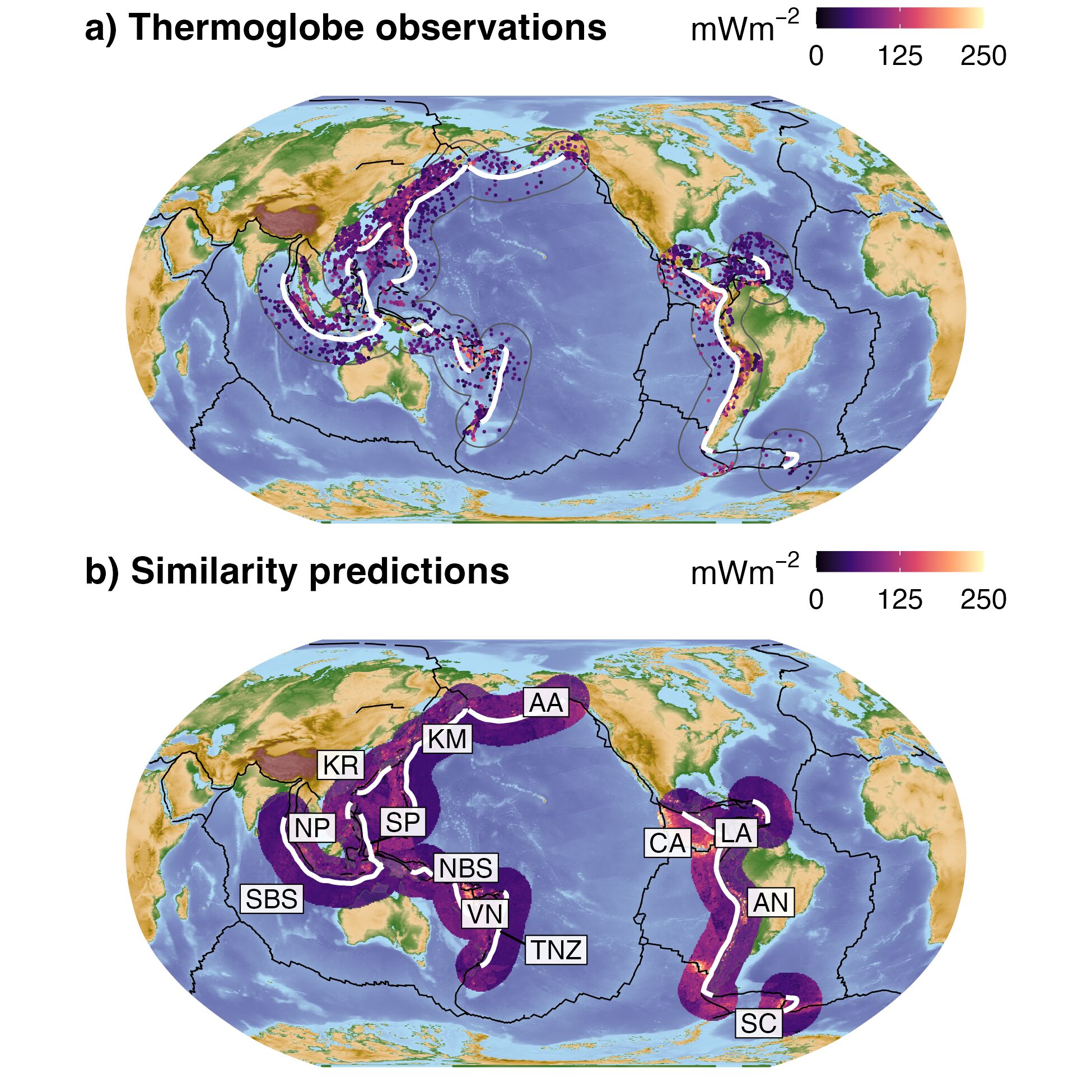
Figure 3.1: Regional surface heat flow near subduction zone segments. (a) ThermoGlobe data from Lucazeau (2019) cropped within 1000 km-radius buffers around 13 active subduction zone segments show uneven regional coverage. For example, note the relatively high observational density in the NW Pacific compared to other regions. (b) In contrast, a Similarity interpolation cropped within the same buffers presents an evenly-distributed approximation of regional surface heat flow. Similarity interpolation from Lucazeau (2019). Subduction zone boundaries (bold white lines) defined by Syracuse & Abers (2006). Plate boundaries (bold black lines) defined by Lawver et al. (2018). AA: Alaska Aleutians, AN: Andes, CA: Central America, KM: Kamchatka Marianas, KR: Kyushu Ryukyu, LA: Lesser Antilles, NBS: New Britain Solomon, NP: N Philippines, SBS: Sumatra Banda Sea, SC: Scotia, SP: S Philippines, TNZ: Tonga New Zealand, VN: Vanuatu.

The two interpolation methods compared in this study, Kriging and Similarity, are chosen because they represent end-member approaches based on fundamentally different principles and mathematical frameworks. Their comparative differences, therefore, may be important for understanding lithospheric thermal structure, identifying surface heat flow anomalies, evaluating practical limitations of each approach, and developing new methods combining the strengths of Kriging and Similarity techniques.

The rationale for applying Kriging and Similarity methods is embodied in the First and Third Laws of Geography, respectively:

Three Laws of Geography:

1. Everything is related, but nearer things are more related (Krige, 1951; Matheron, 1963)

2. Geographic phenomena are inherently heterogeneous (Goodchild, 2004)

3. Localities with similar geographic configurations share other attributes (Zhu et al., 2018)

Generally speaking, the spatial continuity of surface heat flow reflects variations in lithospheric thermal structure and heat-transferring processes (neglecting variations in radiogenic heat production). For example, broad regions of low surface heat flow on continents outline cratons (Nyblade & Pollack, 1993), anomalously low surface heat flow in oceanic crust implies significant heat extraction by seawater (Fisher & Becker, 2000; Hasterok et al., 2011; Hutnak et al., 2008; Stein & Stein, 1994), and trench-orthogonal surface heat flow profiles imply uniform upper-plate lithospheric thickness (Currie et al., 2004; Currie & Hyndman, 2006; Hyndman et al., 2005) and mechanical coupling depths (Furukawa, 1993; Kerswell et al., 2021; Wada & Wang, 2009) among subduction zones. For Kriging, such patterns and anomalies may be resolved (assuming adequate observational coverage) because Kriging estimation is inherently dependent on the spatial continuity of observed surface heat flow.

In contrast, Similarity may impose different patterns than Kriging because the method only depends on the similarity between two localities in terms of their geographic configuration (the makeup and structure of geographic variables over some spatial neighborhood around a point, Zhu et al., 2018). Rather than interpolating (sensu stricto) like Kriging, Similarity predicts surface heat flow by comparing geographic, geologic, geochronologic, and geophysical information between a target point and the entire ThermoGlobe dataset (see Goutorbe et al., 2011 for method details). In other words, Similarity predictions are fundamentally geologically-reasoned estimates of surface heat flow. For example, two localities have similar surface heat flow if they have similar bathymetry, lithology, proximity to active or ancient orogens, seafloor age, upper mantle shear wave velocity, etc. (Chapman & Pollack, 1975; Davies, 2013; Lee & Uyeda, 1965; Lucazeau, 2019; Sclater & Francheteau, 1970; Shapiro & Ritzwoller, 2004).

This study compares regional Similarity and Kriging interpolations near 13 presently active subduction zones while considering the following questions: (1) how does surface heat flow vary near subduction zones, especially within the upper-plate? (2) How do Kriging and Similarity predictions compare? (3) What do the differences (if any) imply about geodynamic variability among active subduction zones? First, ordinary Kriging is applied to ThermoGlobe data near 13 presently active subduction zone segments (defined by Syracuse & Abers, 2006). Kriging predictions are then directly compared (point-by-point) to Similarity predictions from a previous global-scale study by Lucazeau (2019). Interpolation comparisons yield a variety of upper-plate surface heat flow distributions and profiles. Potential implications of mixed upper-plate profiles are discussed, especially with respect to uniform lithospheric thickness (e.g. Currie et al., 2004; Currie & Hyndman, 2006; Hyndman et al., 2005).

3.2 Methods

3.2.1 The ThermoGlobe Database

The ThermoGlobe database is available from the supplementary material of Lucazeau (2019) and is accessible online at http://heatflow.org (Jennings et al., 2021). It currently contains 69,729 data points, their locations in latitude/longitude, and important metadata—including a data quality rank (Code 6) from A (high-quality) to D (low-quality). Lucazeau (2019) and http://heatflow.org provide details on compilation, references, historical perspective on ThermoGlobe, and previous compilations. ThermoGlobe is the most recent database available, has been carefully compiled, and is open-access.

Like Lucazeau (2019), 4,661 poor quality observations (Code 6 = D), 350 data points without heat flow observations, and 2 without geographic information were excluded from the analysis. Note that quality control of such a large dataset is an ongoing endeavor and 11,712 observations currently have an undetermined quality (Code 6 = Z). Duplicate observations at the same location were parsed (to avoid singular covariance matrices during Kriging) by selecting only the best quality measurement. If duplicate measurements were of equal quality, one was randomly chosen. Finally, surface heat flow observations for Kriging and Similarity predictions were both limited to the range (0 - 250] mW/m\(^2\). Observations outside of the range (0 - 250] mW/m\(^2\) are considered anomalous (e.g. collected near geothermal systems, Lucazeau, 2019) and unrepresentative of lithospheric-scale thermal structure. Anomalous observations constitute a small fraction of measurements (4,883 out of 69,729) forming long tails on either side of the global surface heat flow distribution. The final dataset used for Kriging contains 13,360 observations after filtering for quality, missing values, and heat flow range, parsing duplicate pairs, and cropping within subduction zone buffers (Figure B.3 & Table B.2).

3.2.2 Map Projection and Interpolation Grid

All geographic operations, including transformation, cropping, Kriging, and comparing interpolations, were performed using general-purpose functions in the R package sf (Pebesma, 2018). ThermoGlobe data and Similarity interpolations from Lucazeau (2019) were transformed into a Pacific-centered Robinson coordinate reference system using the open source geographic transformation software PROJ (PROJ contributors, 2021). The transformation is defined by the proj4 string "+proj=robin +lon_0=-155 +lon_wrap=-155 +x_0=0 +y_0=0 +ellps=WGS84 +datum=WGS84 +units=m +no_defs". The Kriging domains were defined by drawing 1000 km-radius buffers around each subduction zone segment defined by Syracuse & Abers (2006). Target locations for Kriging (the interpolation grid) were defined across the same grid used by Lucazeau (2019) to compute point-by-point differences with their Similarity interpolation (Figure 3.2). In this case, grid point locations represent the centroids of 0.5˚ \(\times\) 0.5˚ unequal-area grid cells encompassing the entire globe.

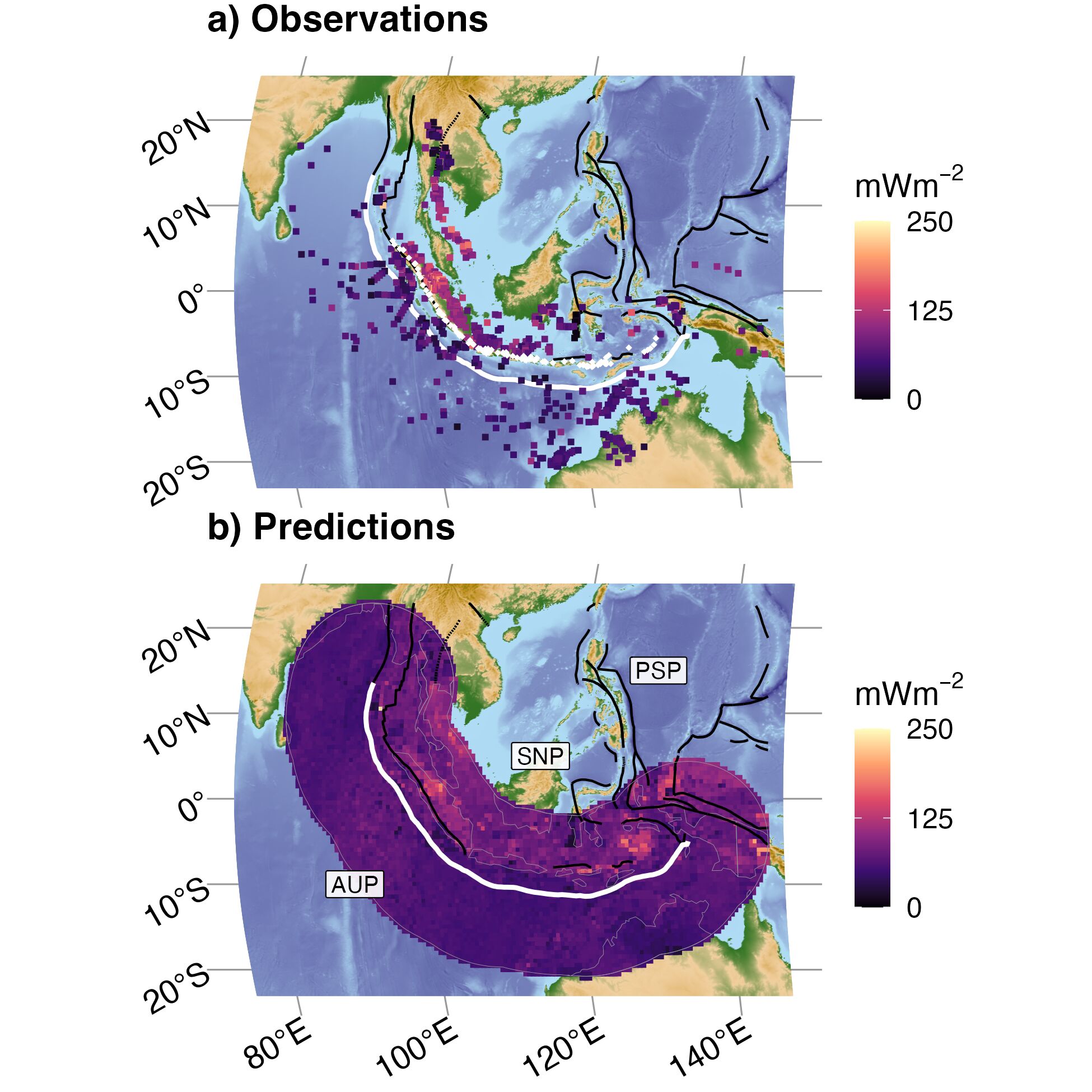
Figure 3.2: Example of an interpolation domain constructed around the Sumatra Banda Sea segment. ThermoGlobe data (colored squares; from Lucazeau, 2019) are cropped within a 1000 km-radius buffer (thin black line) surrounding the segment boundary (bold white line). Target locations for interpolation are defined by the intersections of a 0.5˚ \(\times\) 0.5˚ grid (fine black mesh; defined by Lucazeau, 2019) cropped to the same buffer. Note that Sumatra Banda Sea is one of the more densely sampled regions, yet still has considerable observational gaps. Segment boundary and volcanoes (gold diamonds) defined by Syracuse & Abers (2006). Plate boundaries (bold black lines) defined by Lawver et al. (2018). AUP: Australian Plate, PSP: Philippine Sea Plate, SNP: Sunda Plate.

3.2.3 Kriging

Kriging is derived from the theory of regionalized variables (Matheron, 1963, 2019) and estimates an unknown quantity as a linear combination of all nearby known quantities. Kriging is a three-step process that involves: 1) estimating an experimental variogram \(\hat{\gamma}(h)\) that characterizes the spatial continuity of some quantity within the Kriging domain, 2) fitting one of many variogram models \(\gamma(h)\) to the experimental variogram, and 3) directly solving a linear system of Kriging equations to predict unknown quantities at arbitrary target locations (Cressie, 2015; Krige, 1951). The general-purpose functions defined in the R package gstat (Gräler et al., 2016; Pebesma, 2004) were used to perform all three Kriging steps. The first step computed an experimental variogram (after Bárdossy, 1997): \[\begin{equation} \begin{aligned} \hat{\gamma}(h) &= \frac{1}{2N(h)}\sum_{N(h)}^{}[Z(u_i) - Z(u_j)]^2 \\ h &= |u_i - u_j| \\ \end{aligned} \tag{3.1} \end{equation}\] where \(Z(u_i)\) and \(Z(u_j)\) are observations located at \(u_i\) and \(u_j\) separated by a lag of \(h\), and \(N(h)\) is the number of observations separated by a given lag distance. The experimental variogram \(\hat{\gamma}(h)\) evaluates the spatial continuity of the set of observations \(Z(u)\) by computing the average variance among pairs of observations separated by increasingly greater lag distances. By convention the average variance is halved and called “semivariance”.

For regularly-spaced data, lag distances are simply multiples of the grid-step distance, but irregularly-spaced data must be treated differently. In the case of irregularly-spaced surface heat flow in this study, a binwidth \(\delta\) was defined as: \[\begin{equation} \begin{aligned} &\delta = \frac{\max(h)\ (n_{lag}+shift)}{n_{lag}\ cut} \\ &N(h) = \#\{h \ \in \ [h - \delta,\ h + \delta)\} \end{aligned} \tag{3.2} \end{equation}\] where \(\max(h)\) is the maximum separation distance within the Kriging domain, \(n_{lag}\) is the number of lags used to evaluate the variogram, \(shift\) is a lag shift constant that shifts the variogram by an integer number of binwidths, \(cut\) is a lag cutoff constant (by convention \(cut\) = 3). \(N(h)\) is the number of observations that fall within \([h-\delta,\ h+\delta)\).

This study applied ordinary Kriging with isotropic variogram models (assumes semivariance is spatially invariant) to surface heat flow data projected onto a smooth sphere (neglects elevation). Kriging was applied locally (to avoid violating stationarity assumptions) by evaluating only the nearest \(n_{max}\) observations at each target location, where “nearest” is defined by the distances between the target location and observations. Therefore, the domain of local Kriging expands or shrinks depending on the local observational density at each target location.

Several variogram parameters influence the Kriging result, including the choice of variogram model, the scope of local Kriging \(n_{max}\), and choice of experimental variogram parameters in Equation (3.1). Instead of choosing Kriging parameters by eye (a common practice for fitting variograms) this study used a constrained non-linear optimization approach to find optimum values for the variogram parameters \(\{model,\ n_{lag},\ cut,\ n_{max},\ shift\}\). A weighted sum of the RMSE evaluated during variogram fitting and the RMSE evaluated between Kriging estimates and surface heat flow observations was used as a cost function to simultaneously optimize variogram and Kriging accuracy (after Li et al., 2018). The R package nloptr was used to optimize Kriging parameters by finding a combination of the parameters \(\{model,\ n_{lag},\ cut,\ n_{max},\ shift\}\) that minimizes the cost function. A full description of the Kriging system of equations, underlying assumptions, and optimization methods is presented in Appendix B.1 with optimization results for all segments and variogram models. All experimental and fitted variograms are in Appendix B.4 with interpolations for each case not presented in the main text.

3.2.4 Upper-Plate Sector Profiles

Surface heat flow profiles and distributions were computed for several adjacent upper-plate regions to assess lateral (along-strike) surface heat flow variability. Profiles were defined by (1) splitting a subduction zone segment (defined by Syracuse & Abers, 2006) into 2-14 equidistant parts, (2) defining 500 km-wide single-sided buffers (sectors) around the segment parts, and (3) calculating the orthogonal great circle distance between each surface heat flow prediction (Similarity and Kriging), or observation (ThermoGlobe data), contained within a sector and the segment boundary (trench). Steps (1-3) above closely approximate the projection of surface heat flow onto a 1D trench-orthogonal line at the center of each sector (e.g. Currie et al., 2004; Currie & Hyndman, 2006; Hyndman et al., 2005; Morishige & Kuwatani, 2020; Wada & Wang, 2009). Profiles were smoothed by a three-point running average and fit with a local non-parametric regression curve (LOESS, Cleveland & Devlin, 1988).

3.2.5 Interpolation Accuracy

Previous studies evaluate global Similarity accuracy by either applying cross-validation during the interpolation process (e.g. Goutorbe et al., 2011) or directly computing residuals between predictions and surface heat flow observations after interpolation (e.g. Lucazeau, 2019). Generally speaking, ranking models by comparing cross-validation results is typically preferred over directly comparing residuals for two reasons: (1) cross-validation gives a sense of how a model behaves when presented with new data (not part of the training data set used to fit the model), and (2) cross-validation can distinguish models that are overfit (high-accuracy due to “memorizing” the training data set). However, because Similarity is a non-parametric approach that does not involve “fitting” models to sets of training data (i.e. no residuals or cost function to minimize), cross-validating Similarity predictions does not effectively distinguish overfitting, nor does it give a sense of how well Similarity will behave when presented with new data. Similarity, as typically implemented (e.g. by Goutorbe et al., 2011; Lucazeau, 2019), always considers the entire global dataset of surface heat flow observations to make predictions at unknown target locations. Therefore leaving out a few observations has little effect. For example, even removing an entire continent’s worth of surface heat flow data does not significantly affect the outcome of Similarity predictions compared to Similarity interpolations including the full ThermoGlobe dataset (see Figure 9 in Lucazeau, 2019).

To better compare Kriging (a parametric model fit to training data) and Similarity (a non-parametric model with prescribed weights), this study computed interpolation accuracies using a direct approach (similar to Lucazeau, 2019) for both methods. More specifically, the RMSE was computed for each surface heat flow observation by comparing the observed value to the nearest predicted value made across the 0.5˚ \(\times\) 0.5˚ interpolation grid. Compared to cross-validation, this direct method provides a more robust and effective comparison between Similarity and Kriging accuracies. However, the direct approach is particularly susceptible to ignoring overfitting during Kriging estimation. Therefore caution must be taken to avoid misinterpreting unusually low Kriging error rates as indication of a more accurate model.

3.3 Results

3.3.1 Global Differences

Global differences between Similarity and Kriging interpolations across all subduction zone segments are centered near zero with median differences ranging from -1 to 14 mW/m\(^2\), but broadly distributed with IQRs from 15 to 50 mW/m\(^2\) and long tails extending from -1000 to 205 mW/m\(^2\) (Table B.3). Distributions of interpolation differences are either approximately symmetrical, or slightly right-skewed (Figure B.4). Slight right skew and positive median differences indicate a general tendency to predict higher surface heat flow by Similarity compared to Kriging. However, much of the right skew can be explained by spreading centers, transform faults, and volcanic regions predicted by Similarity that are unresolved by Kriging due to lack of observations in those regions (e.g. Scotia), and/or regions of anomalously-low surface heat flow within oceanic crust resolved by Kriging that are effectively overlooked by Similarity (e.g. Central America).

3.3.2 Regional Differences

Examples given in this section highlight the range of differences observed between Similarity and Kriging interpolations across subduction zone segments with anomalously-low surface heat flow within oceanic crust (Central America), with complex tectonic boundaries (Vanuatu), with excellent observational coverage (Kyushyu Ryukyu), and with very few observations (Scotia). Refer to Appendix B.4 for the remaining set of visualized interpolations.

3.3.2.1 Central America

Distance to plate boundaries and the age of oceanic lithosphere are key geologic proxies exerting strong influence on Similarity predictions (Goutorbe et al., 2011; Shapiro & Ritzwoller, 2004; Stein & Stein, 1992). Consequently, Similarity predicts high surface heat flow along the arms of the Galápagos triple junction and within the (young) converging Cocos Plate near Central America (Figure 3.3). Kriging, on the other hand, predicts relatively low surface heat flow within the Cocos Plate despite its young age and close proximity to the nearby spreading centers. This is explained by anomalously-low surface heat flow observed within the Cocos Plate that is interpreted as regional modification of the expected surface heat flow by hydrothermal circulation of seawater (Hutnak et al., 2008). These widespread observations of low surface heat flow constrain Kriging predictions to similarly low values within the Cocos Plate. Disagreement between Similarity and Kriging appears more subdued within the upper-plate, yet Similarity still predicts slightly higher surface heat flow on average.

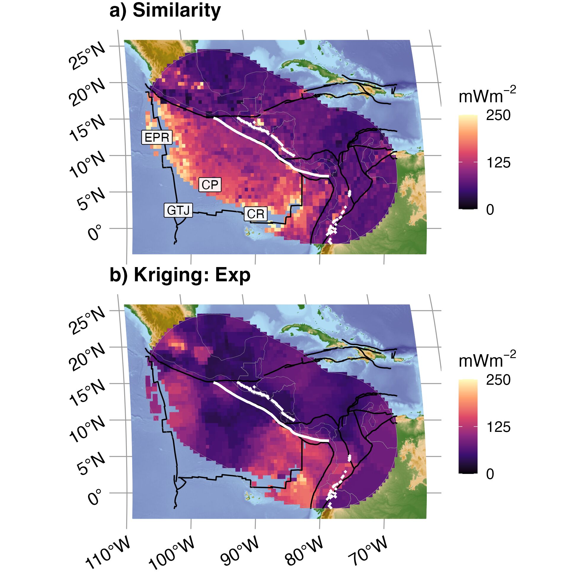
Figure 3.3: Similarity and Kriging interpolations for Central America. (a) Relatively high surface heat flow is predicted by Similarity within the young Cocos Plate (CP) and along the arms of the Galápagos triple junction (GTJ): the East Pacific Rise (EPR) and Cocos Ridge (CR). In contrast, (b) many anomalously-low surface heat flow observations within the CP (Hutnak et al., 2008) constrain Kriging predictions to low values. Segment boundary (bold white line) and volcanoes (gold diamonds) defined by Syracuse & Abers (2006). Similarity interpolation from Lucazeau (2019). Plate boundaries (bold black lines) defined by Lawver et al. (2018).

3.3.2.2 Vanuatu

The interpolation domain near Vanuatu is characterized by complex tectonic boundaries defining several microplates to the east of the volcanic arc (Figure 3.4). The resolution of the geologic proxy datasets used to construct Similarity predictions (namely oceanic plate age, upper mantle density anomaly, sediment thickness, and distance to tectonic boundaries) is apparently too coarse to distinguish a small microplate near the northern tip of the Vanuatu segment from the New Hebrides, Balmoral Reef, and Conway Reef microplates. According to Similarity, the entire region is comprised of young oceanic plate with thin sediment cover, and thus is predicted to have uniformly-high surface heat flow. In contrast, excellent observational coverage enables Kriging to clearly distinguish the northern microplate as an anomalously-low surface heat flow region compared to the other microplates. Outside the cluster of microplates, Kriging predicts lower surface heat flow on average—similar to many other segments.

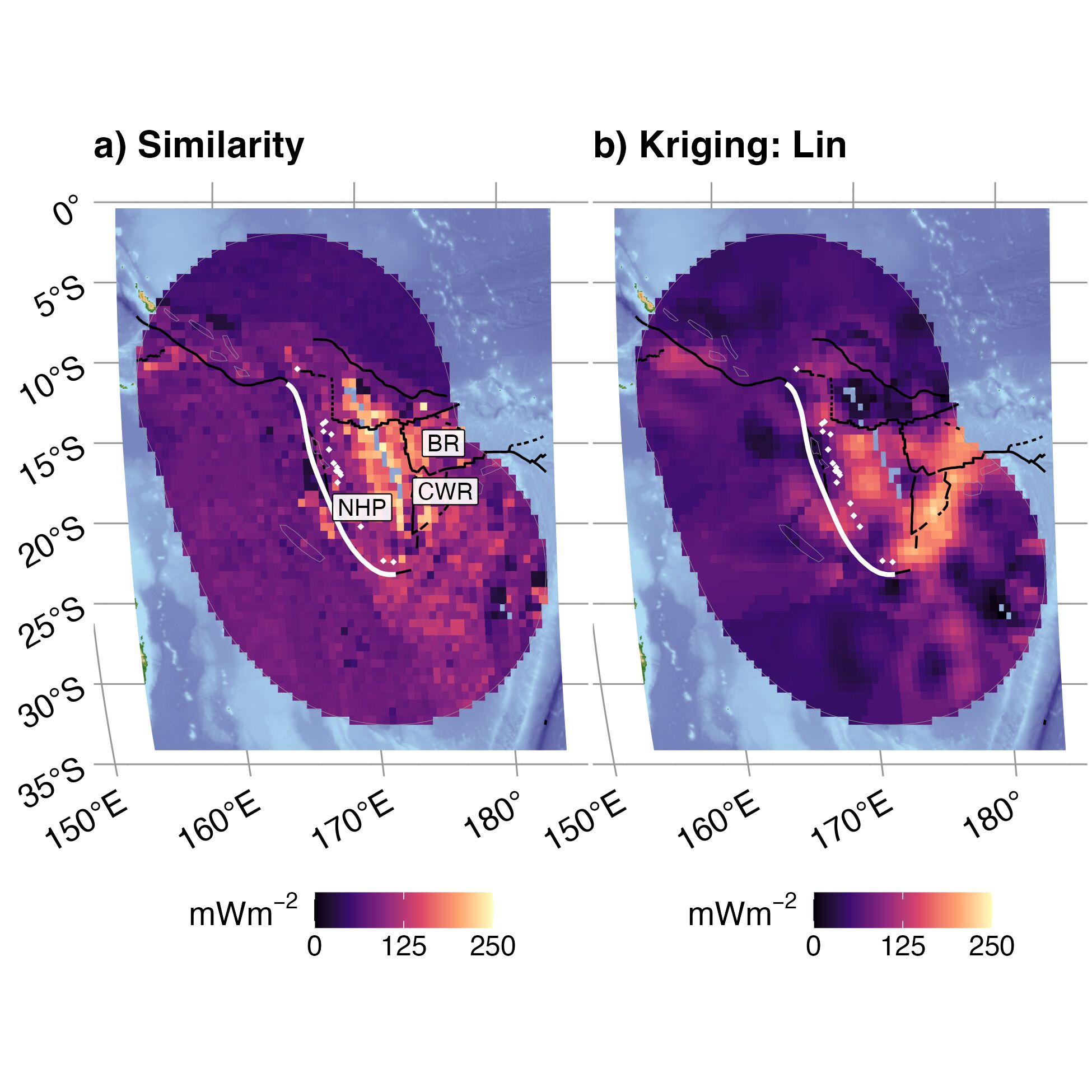
Figure 3.4: Similarity and Kriging interpolations for Vanuatu. While (a) Similarity predicts more-or-less uniformly-high surface heat flow within the region defined by many microplates, (b) excellent observational coverage allows Kriging to distinguish the most northern microplate from the New Hebrides Plate (NHP), Balmoral Reef (BR), and Conway Reef (CWR) microplates to the S. The geologic proxy datasets used to construct Similarity interpolations are apparently too coarse to resolve microplate-size features in this case. Segment boundary (bold white line) and volcanoes (gold diamonds) defined by Syracuse & Abers (2006). Similarity interpolation from Lucazeau (2019). Plate boundaries (bold black lines) defined by Lawver et al. (2018).

3.3.2.3 Kyushu Ryukyu

The interpolation domain near the Kyushu Ryukyu segment is characterized by a complex juxtaposition of active subduction and volcanism on the margins of the Philippine Sea Plate, and active rifting between the Ryukyu arc and the Eurasian continent (the Okinawa trough, Minami et al., 2022). Contrasting oceanic plate ages, topography/bathymetry, sediment thickness, volcanic activity, and active tectonic settings (subduction vs. rifting) consequently produce a very textured distribution of Similarity predictions throughout the Kyushu Ryukyu domain (Figure 3.5). For example, Similarity predictions clearly show the influence of multiple volcanic arc chains, plate boundaries, and the age of the subducting oceanic lithosphere. Geologic complexity notwithstanding, excellent coverage of surface heat flow observations throughout the domain enable Kriging predictions to resolve much of the texture predicted by Similarity. Regional Similarity and Kriging differences are small and narrowly distributed near Kyushu Ryukyu (median difference: 4, IQR: 21 mW/m\(^2\)) as compared, for example, to Central America (median difference: 12, IQR: 50 mW/m\(^2\); Table B.3) despite having a comparable number of observations (n = 1,895) as Central America (n = 1,441). While Kriging predictions are smoother overall, both interpolations appear to corroborate each other, especially to the NE of the main Kyushu Ryukyu segment boundary.

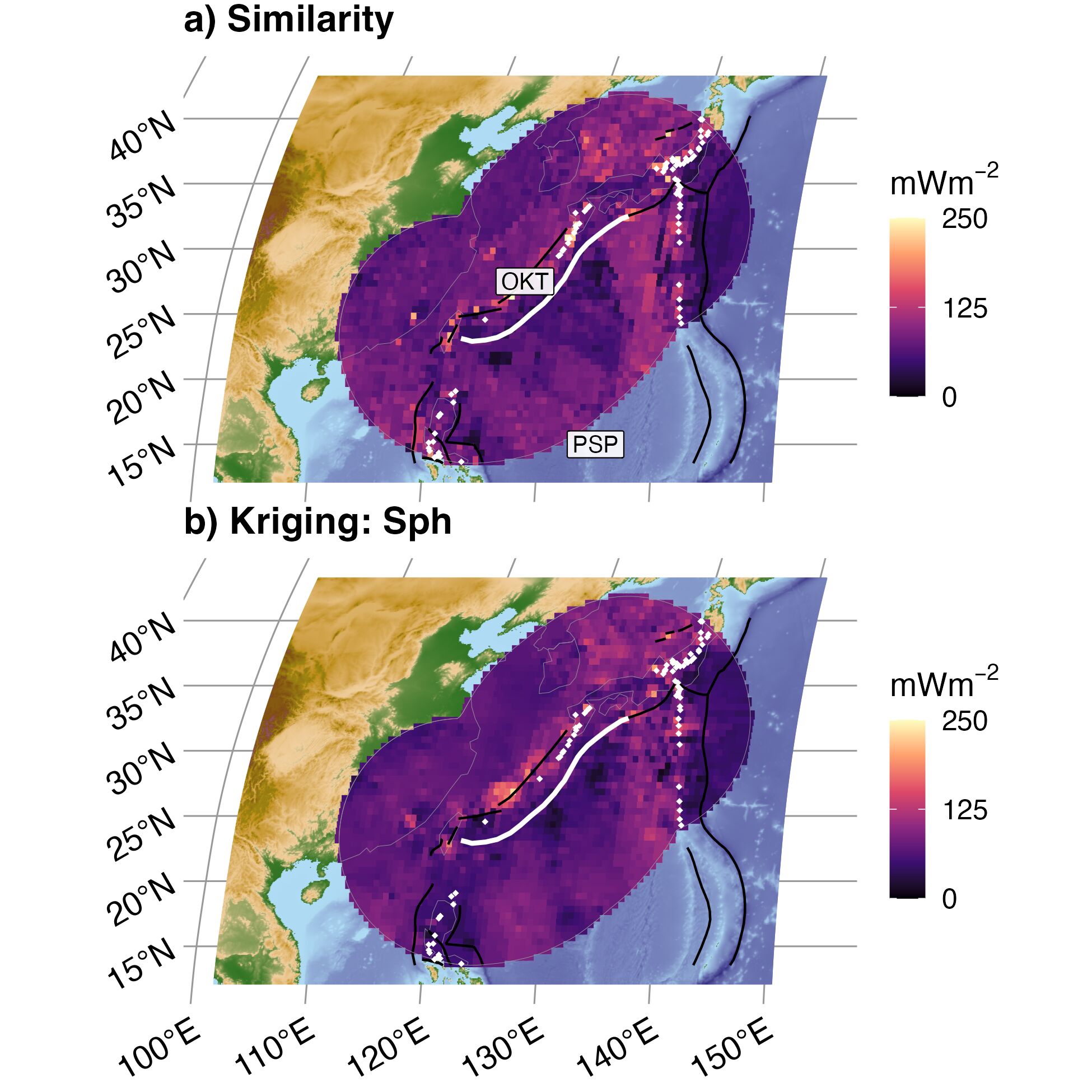
Figure 3.5: Similarity and Kriging interpolations for Kyushyu Ryukyu. (a) Similarity predicts a textured interpolation that is strongly influenced by multiple volcanic chains along the margins of the Philippine Sea Plate (PSP), contrasting oceanic plate ages, and active rifting in the Okinawa trough (OKT). (b) The Kriging interpolation is generally smoother, but corroborates much of the same texture predicted by Similarity due to relatively high observational density and regularity of observational coverage throughout the domain. Segment boundary (bold white line) and volcanoes (gold diamonds) defined by Syracuse & Abers (2006). Similarity interpolation from Lucazeau (2019). Plate boundaries (bold black lines) defined by Lawver et al. (2018).

3.3.2.4 Scotia

The Scotia segment illustrates a case where surface heat flow observations are extremely sparse. Yet Similarity predicts multiple tectonic features including the East Scotia Ridge and the WSW-ENE trending transform boundary separating the Scotia and Sandwich Plates from the Antarctic Plate (Figure 3.6). Combinations of geologic proxy datasets enable Similarity to resolve these features despite having very few observations within the interpolation domain. Kriging, on the other hand, shows a high heat flow anomaly more or less in the region of the East Scotia Ridge, and a few low heat flow anomalies on the Antarctic Plate, but does not resolve any structure in a way that is geologically useful. Few surface heat flow observations (n = 25) result in smooth Kriging predictions that approximate the expected mean value (79 mW/m\(^2\)) for most of the domain according to Equation (B.3).

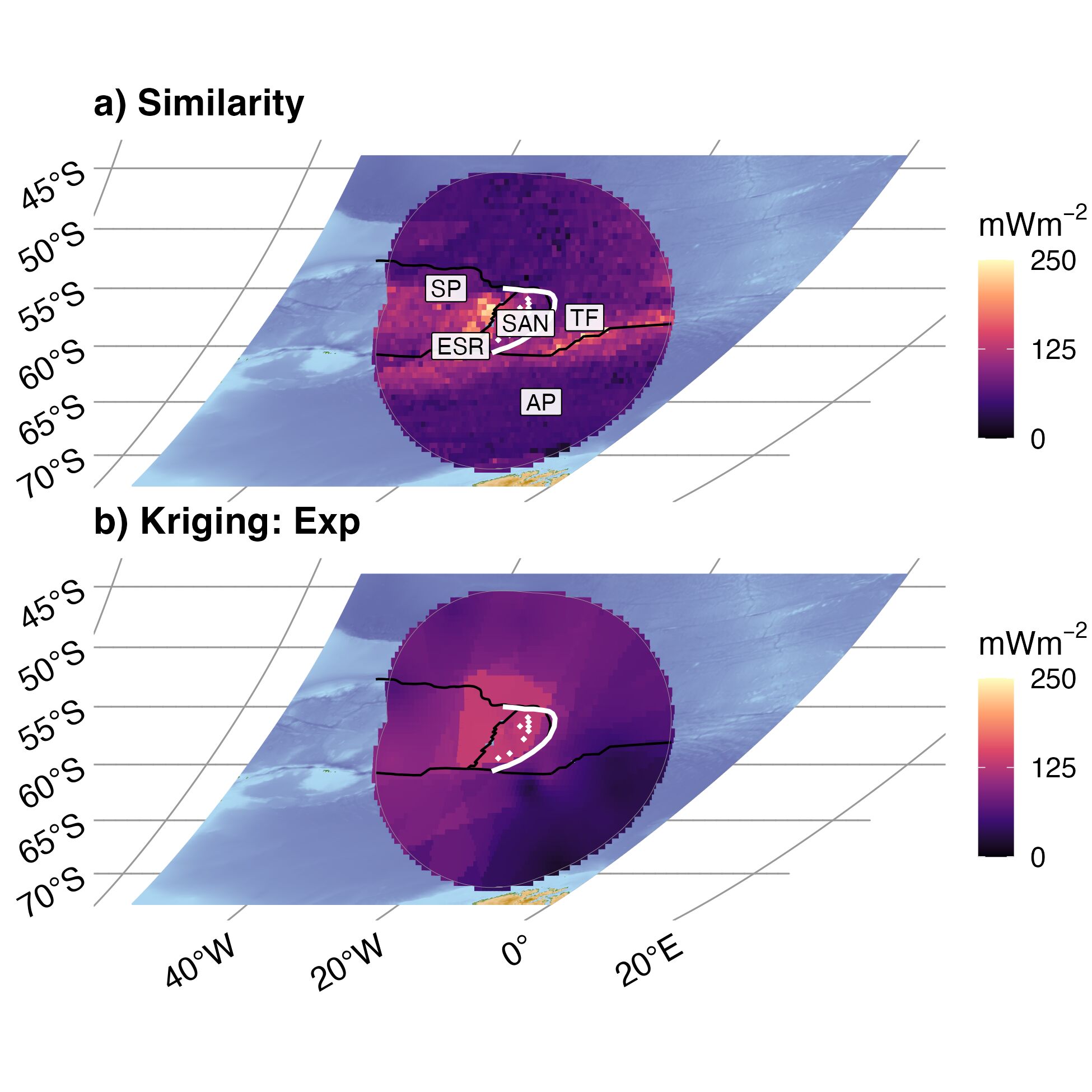
Figure 3.6: Similarity and Kriging interpolations for Scotia. Despite extremely sparse data (n = 25), (a) Similarity identifies two tectonic features, the East Scotia Ridge (ESR) and a transform fault (TF) separating the Scotia and Sandwich Plates (SP, SAN) from the Antartic Plate (AP). (b) Kriging predicts a high heat flow anomaly in the region of the ESR, and a few low heat flow anomalies in the AP, but otherwise appears featureless due to sparse data. Segment boundary (bold white line) and volcanoes (gold diamonds) defined by Syracuse & Abers (2006). Similarity interpolation from Lucazeau (2019). Plate boundaries (bold black lines) defined by Lawver et al. (2018).

3.3.3 Upper-Plate Sector Samples

Sampling the interpolation grid and ThermoGlobe data from adjacent upper-plate sectors allows for first-order quantitative evaluation of the along-strike variability in upper-plate surface heat flow. However, ThermoGlobe data within sectors are often too few (n < 20 observations for 59/100 sectors; Table B.5) to compare distributions confidently with other sectors. Therefore, this study compares trench-orthogonal profiles of the dense, regularly-spaced Similarity and Kriging predictions. Generally speaking, distributions of Similarity and Kriging predictions in the upper-plates show a range of overlap and appear to fluctuate systematically across adjacent upper-plate sectors for some subduction zone segments. Moreover, Similarity and Kriging predictions reveal a variety of upper-plate surface heat flow profiles within and among subduction zone segments (Table B.5, Figures 3.7, 3.8, 3.9 & Appendix B.5).

Below are three examples of subduction zone segments that illustrate part of the range of observed upper-plate surface heat flow patterns.

3.3.3.1 Kyushu Ryukyu

Kyushu Ryukyu characterizes a subduction zone segment with relatively consistent upper-plate surface heat flow for thousands of km along-strike. In this case, consistent refers to comparable Similarity and Kriging predictions and consistent surface heat flow distributions across sectors. That is, medians and IQRs of Similarity and Kriging predictions overlap relatively well across most sectors—differing by only 6.4 ± 10.2 mW/m\(^2\) for medians and 19.9 ± 34 mW/m\(^2\) for IQRs, on average (Table B.5 & Figure 3.7). Upper-plate surface heat flow, as estimated by Kriging, appears to increase systematically from the NE to SW across sectors 8-6 before leveling out through sectors 5-1.

Meanwhile, ThermoGlobe data within Kyushu Ryukyu upper-plate sectors (n = 339) vary considerably. Wide distributions of ThermoGlobe data appear near the trench and at approximately 200 km from the trench, coinciding with the young active rifting in the Okinawa trough (Figure 3.7). Yet, smoothed trench-orthogonal Similarity and Kriging profiles gently arc through the approximate midrange of ThermoGlobe data. Profile shapes are consistent across sectors and show relatively little spread (\(\leq\) 25 mW/m\(^2\)). All profiles gradually rise from approximately 50 mW/m\(^2\) at the trench to maximums of approximately 75-100 mW/m\(^2\) before gradually decreasing to approximately 75 mW/m\(^2\) at 500 km into the upper-plate.

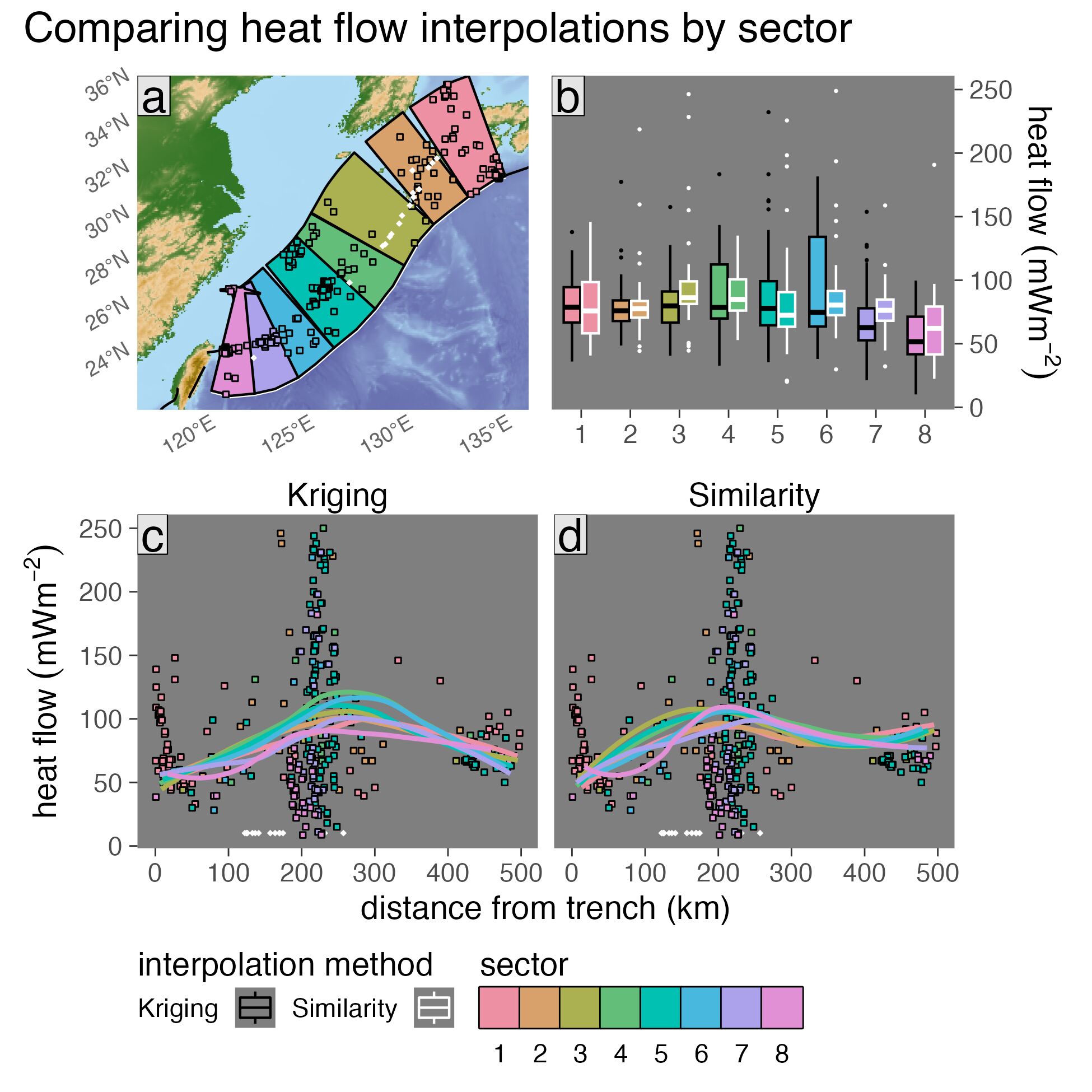
Figure 3.7: Surface heat flow profiles for Kyushu Ryukyu upper-plate sectors. (a) Similarity and Kriging predictions across sectors are largely indistinguishable with overlapping medians and IQRs (boxes). (b) Profiles are computed by finding orthogonal distances between the segment boundary (i.e. the trench, bold black line) and 342 surface heat flow predictions within eight 500 km-wide sectors (colored polygons). Profiles (colored curves with 95% confidence intervals) are remarkably consistent across sectors for (c) Kriging and (d) Similarity predictions. Colored squares are ThermoGlobe data from Lucazeau (2019). Segment boundary and volcanoes (gold diamonds) defined by Syracuse & Abers (2006). Plate boundaries (bold black lines) defined by Lawver et al. (2018). Profile curves in (c) are LOESS regressions through three-point running averages (small colored data points).

3.3.3.2 Sumatra Banda Sea

Sumatra Banda Sea characterizes a subduction zone segment with moderately consistent upper-plate surface heat flow for thousands of km along-strike. In this case, moderately consistent refers to mostly comparable (overlapping) Similarity and Kriging predictions that distinctively fluctuate in a similar manner across sectors. That is, medians and IQRs of Similarity and Kriging predictions overlap well for some sectors, but not others (e.g. sectors 1, 10, & 11, Figure 3.8). Median Similarity and Kriging predictions differ by 10.7 ± 14.2 mW/m\(^2\) on average, and IQRs differ by 17.3 ± 61.2 mW/m\(^2\) on average across all sectors (Table B.5). Similarity and Kriging predictions appear to broadly oscillate between higher and lower surface heat flow across adjacent sectors with a wavelength on the order of several sectors (10\(^3\) km).

Meanwhile, Similarity and Kriging profiles show obvious differences. For example, Similarity predictions are distributed narrowly and increase monotonically from the trench to 500 km into the upper-plate, whereas Kriging profiles generally ramp up more steeply and begin to disperse at approximately 200 km from the trench. Similarity profiles remain narrowly distributed through at least 300 km from the trench, whereas Kriging profiles show up to 25-30 mW/m\(^2\) spread among sectors at 300-500 km from the trench.

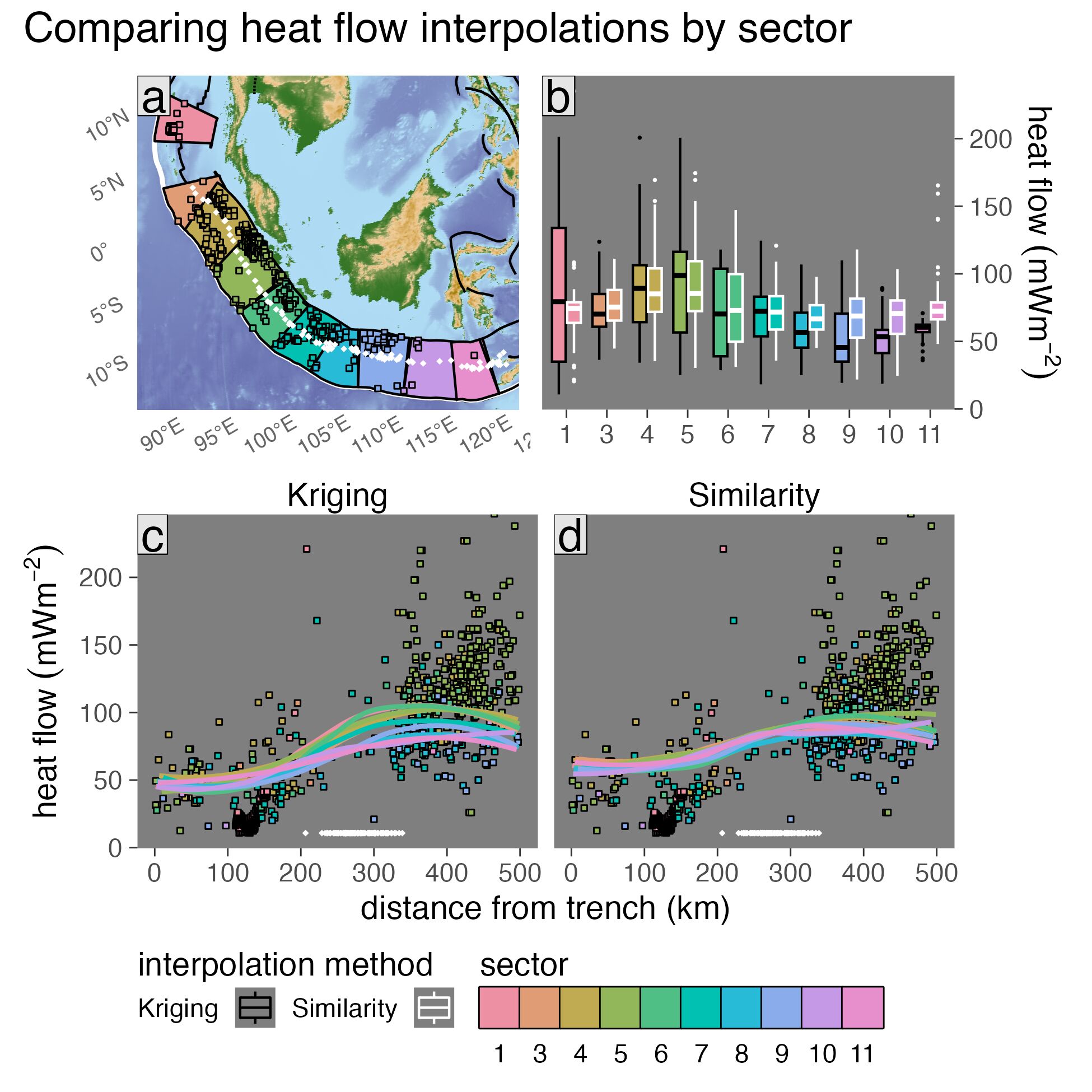
Figure 3.8: Surface heat flow profiles for Sumatra Banda Sea upper-plate sectors. (a) Similarity and Kriging predictions across sectors are moderately distinguishable with mostly overlapping IQRs, except for sectors 1, 10, & 11 (boxes). (b) Profiles are computed by finding orthogonal distances between the segment boundary (trench; bold black line) and 870 surface heat flow predictions within ten 500 km-wide sectors (colored polygons). Profiles (colored curves with 95% confidence intervals) of (c) Kriging predictions show greater overall spread than (d) Similarity profiles (e.g. \(\geq\) 200 km from the trench), implying nonuniform upper-plate surface heat flow across the segment. Colored squares are ThermoGlobe data from Lucazeau (2019). Segment boundary and volcanoes (gold diamonds) defined by Syracuse & Abers (2006). Plate boundaries (bold black lines) defined by Lawver et al. (2018). Profile curves in (c) are LOESS regressions through three-point running averages (small colored data points).

3.3.3.3 New Britain Solomon

New Britain Solomon characterizes a subduction zone segment with inconsistent upper-plate surface heat flow and poor overlap between Similarity and Kriging predictions. Only one sector (sector 8) shows overlapping IQRs of Similarity and Kriging predictions, whereas all other sectors strongly diverge (Figure 3.9). For example, median Kriging predictions range by 21.4 mW/m\(^2\) across all sectors, whereas median Similarity predictions range by 42.7 mW/m\(^2\). Moreover, Similarity and Kriging medians across all sectors differ by 32.4 ± 50.2 mW/m\(^2\) on average. Notably, opposing wave-like oscillations between higher and lower surface heat flow across adjacent sectors are observed in Similarity and Kriging predictions.

Meanwhile, Similarity and Kriging profiles are obviously distinguishable. For example, Kriging profiles are smooth and closely parallel ThermoGlobe data, whereas Similarity profiles show higher average surface heat flow (Figure 3.9). In contrast to flat Kriging profiles, high surface heat flow regions along Similarity profiles clearly show the influence of certain tectonic features (e.g. in sector 4, which intersects a volcanic center and ridge segment). Moreover, small confidence intervals around Kriging profiles suggest small uncertainties compared to Similarity. However, Kriging is determined to find the smallest variance solution by definition and can easily overfit the small number (n = 9) of ThermoGlobe data. Divergence between Similarity and Kriging predictions near New Britain Solomon thus appear to be driven by methodological differences and a tendency for Kriging to overfit small sample sets.

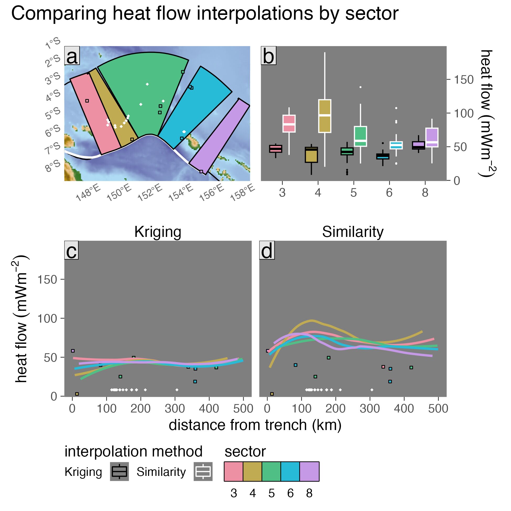
Figure 3.9: Surface heat flow profiles for New Britain Solomon upper-plate sectors. (a) Similarity and Kriging predictions across sectors are very distinguishable with non-overlapping IQRs (boxes). (b) Profiles are computed by finding orthogonal distances between the segment boundary (trench; bold black line) and 163 surface heat flow predictions within five 500 km-wide sectors (colored polygons). Profiles (colored curves with 95% confidence intervals) of (c) Kriging predictions are lower and show a narrow distribution compared to (d) Similarity profiles. Colored squares are ThermoGlobe data from Lucazeau (2019). Segment boundary and volcanoes (gold diamonds) defined by Syracuse & Abers (2006). Plate boundaries (bold black lines) defined by Lawver et al. (2018). Profile curves in (c) are LOESS regressions through three-point running averages (small colored data points).

3.3.4 Optimum Kriging Parameters

Optimized Kriging parameters vary substantially from segment to segment (Table 3.1). However, despite a range of domain sizes, observational densities, and diverse plate configurations, Kriging parameters converge on solutions for all Kriging domains (Figure B.2) and show no systematic correlation with cost, with the exception of a negative correlation with the logarithm of the variogram model sill (Figure B.1). Differences in cost are apparently explained by systematic regional differences in surface heat flow distributions (i.e. differences in the constant terms \(\sigma_{vgrm}\) and \(\sigma_{interp}\) in Equation (B.8)) rather than sensitivity to any particular Kriging parameter.

Table 3.1: Optimum variogram models and interpolation accuracy

Segment	Model	Cut	Lags	Shift	\(n_{max}\)	Sill	Range	\(RMSE_S\)	\(RMSE_K\)
						\((mW/m^2)^2\)	km	mW/m\(^2\)	mW/m\(^2\)
Alaska Aleutians	Bes	1.0	16.3	1.0	8	841	77	17.6	74.6
Andes	Exp	1.6	20.8	8.5	12	4631	165	52.6	34.9
Central America	Exp	4.9	21.2	3.9	12	4683	265	52.5	33.4
Kamchatka Marianas	Sph	1.7	18.5	7.5	7	1787	1355	33.1	31.2
Kyushu Ryukyu	Lin	3.2	19.8	3.3	8	1898	183	34.5	37.8
Lesser Antilles	Lin	1.5	24.2	1.1	11	653	77	11.5	13.3
N Philippines	Bes	1.4	18.3	1.0	8	1258	19	27.1	32.0
New Britain Solomon	Lin	2.0	20.2	5.1	10	693	228	13.6	28.2
S Philippines	Lin	3.2	29.0	1.0	5	1014	40	25.6	22.9
Scotia	Sph	2.7	20.8	4.8	8	3655	1766	26.5	10.9
Sumatra Banda Sea	Sph	6.6	21.0	5.1	13	10598	5850	18.0	20.4
Tonga New Zealand	Lin	3.7	24.9	3.6	10	1293	321	24.1	23.8
Vanuatu	Lin	1.2	20.4	2.6	11	2918	286	37.1	54.6
note: showing lowest-cost models from Table B.1
key: \(n_{max}\): max point-pairs, \(RMSE_S\): Similarity accuracy, \(RMSE_K\): Kriging accuracy

3.3.5 Similarity and Kriging Error Rates

Regional Kriging error rates (ranging from 10.9 to 74.6 mW/m\(^2\)) are very similar to Similarity error rates from the same regions (ranging from 11.5 to 52.6 mW/m\(^2\), Table 3.1). Kriging errors can be relatively small compared to Similarity for domains with high observational density (e.g. Lesser Antilles; n = 3,008, \(\Delta\)RMSE\(_{K-S}\) = 1.9) but relatively large where observational density is comparatively low (Alaska Aleutians; n = 290, \(\Delta\)RMSE\(_{K-S}\) = 57). The small Kriging error rate computed for Scotia (10.9 mW/m\(^2\)) likely reflects overfitting of few (n = 25) observations. On average, Kriging error rates are 1.3 times Similarity error rates across all segments. In comparison to previous work, regional Similarity error rates for most subduction zone segments in Table 3.1 are much higher than the 7 mW/m\(^2\) Similarity error rate reported by Lucazeau (2019). However, Similarity error rates in Table 3.1 are consistent with global Similarity error rates computed by cross-validation on a 1˚ \(\times\) 1˚ grid (from 11.6 to 29.0 \(mW/m^{-2}\)) reported previously by Goutorbe et al. (2011).

3.4 Discussion

3.4.1 Comparing Similarity and Kriging Interpolations

Comparing two independent interpolation methods has distinct advantages for understanding subduction zone thermal structure and geodynamics. For example, many cases of Similarity and Kriging predictions corroborate known, expected, or predicted tectonic features. These include: (1) broad regions of low surface heat flow defining the oceanic plate and forearc along the Kamchatka Marianas segment (Figure B.8), (2) high surface heat flow anomalies defining the volcanic center and transform fault separating the South American Plate and Caribbean Plates near the Lesser Antilles Segment (Figure B.9), (3) the general seafloor thermal structure near the N Philippines segment (Figure B.10), (4) a broad region of high surface heat flow within the NW part of the Sumatra Banda Sea segment upper-plate (Figure B.13), and (5) high surface heat flow defining volcanic arc chains near the Kyushu Ryukyu segment (Figure 3.5).

While corroboration of known or expected features is advantageous when comparing independent interpolation methods, inconsistencies between Similarity and Kriging predictions are equally valuable. For example, many cases of Similarity and Kriging predictions identify unexpected or poorly resolved tectonic features. These include: (1) much of the thermal structure along the Andes segment (Figure B.7), (2) the location and extent of two spreading centers, the tip of a transform fault, and the regional thermal structure of the Cocos Plate near the Central America segment (Figure 3.3), (3) locations of plate boundaries near the New Britain Solomon (Figure B.11) and Scotia segments (Figure 3.6), (4) a large low surface heat flow anomaly near the Sumatra Banda Sea segment (east of Borneo at approximately 120˚E and 5˚S, Figure B.13), (5) a high heat flow anomaly defining a transform fault near the N tip of the Tonga New Zealand segment (Figure B.14), and (6) the location of microplate boundaries near the Vanuatu segment (Figure 3.4).

Such inconsistencies between Similarity and Kriging interpolations identify tectonic features that either violate geologic proxy datasets, violate local surface heat flow observations, lack sufficient observational coverage to be resolved by Kriging, or are too fine-scale to be resolved by geologic proxy datasets on a 0.5˚ \(\times\) 0.5˚ grid. In any case, the above examples demonstrate the utility of comparing independent interpolation methods in identifying relevant targets for future investigation and data acquisition (discussed further below). Maps of regional interpolated surface heat flow prepared in this study (Section 3.3 and Appendices B.4 & B.5, or similar) therefore provide important context for subduction zone research.

3.4.2 Comparing Upper-Plate Sectors

3.4.2.1 Issues with Irregularly-Spaced Data

Surface heat flow profiles in previous studies were computed with observations sampled from within a single sector (Currie et al., 2004; Currie & Hyndman, 2006; Furukawa, 1993; Hyndman et al., 2005; Kerswell et al., 2021; Wada & Wang, 2009). While extending a single-sector sampling approach to many adjacent sectors is simple to implement, inherent pitfalls are immediately obvious when comparing ThermoGlobe data among sectors. For example, the spatial density and regularity of ThermoGlobe data within adjacent sectors can often be drastically different (e.g. compare ThermoGlobe data counts across sectors from Central America, Sumatra Banda Sea, and Tonga New Zealand in Table B.5). Fluctuating sample sizes among upper-plate sectors can make statistical comparisons of ThermoGlobe data equivocal. For instance, ThermoGlobe data are often too few (n < 20 observations for 59/100 sectors, Table B.5) to compare with statistical confidence. Many sectors (n = 10) have a single observation with a singular distribution (IQR = 0) or few observations spanning a large range (very large IQR). Many sectors encompass zero ThermoGlobe data and therefore cannot be compared at all. In other words, summary statistics necessary for gauging the continuity of surface heat flow among sectors (e.g. median, IQR, Table B.5) can be generally considered unreliable for a majority of sectors.

The above limitation arising from sampling irregularly-spaced data can be easily overcome by interpolation. That is because sampling a regular interpolation grid allows for more consistent sample sizes and spatial coverage across sectors. For example, many sectors defined in this study have few ThermoGlobe data (n < 5 observations for 37/100 sectors, Table B.5), yet the average number of Similarity and Kriging predictions within those same sectors is 51—about 10 times the sample size on average. Surface heat flow variability among sectors is thus more confidently and consistently evaluated with interpolations derived from ThermoGlobe data, rather than from ThermoGlobe data directly.

3.4.2.2 Continuity of Upper-Plate Surface Heat Flow

How consistent and continuous is upper-plate surface heat flow within and among subduction zone segments? While Similarity and Kriging predictions show discontinuous upper-plate surface heat flow patterns for some segments (e.g. Andes, Lesser Antilles and Vanuatu, Figures B.16, B.19 & B.24), other segments show rather continuous patterns (e.g. Central America, Kamchatka Marianas, Kyushu Ryukyu, N Philippines, Figures B.17, B.18, 3.7, B.20), and still other segments show mixed patterns depending on the interpolation method (e.g. Alaska Aleutians, New Britain Solomon, S Philippines, Sumatra Banda Sea, Tonga New Zealand, Figures B.15, 3.9, B.21, 3.8, B.23). On the one hand, Similarity and Kriging interpolations can show nearly identical profiles along-strike for 1000’s of km (e.g. Kamchatka Marianas, Kyushu Ryukyu, Sumatra Banda Sea, Figures B.18, 3.7, 3.8). These segments demonstrate large-scale continuity in upper-plate surface heat flow and may imply spatially homogeneous lithospheric thermal structure and/or spatially homogeneous heat-transferring dynamics (e.g. Currie et al., 2004; Currie & Hyndman, 2006; Furukawa, 1993; Kerswell et al., 2021; Wada & Wang, 2009). Alternatively, continuous surface heat flow may reflect undersampling relative to local spatial variability of surface heat flow. Moreover, most segments show neither completely continuous nor discontinuous upper-plate surface heat flow patterns (Table B.5).

Some segments show an apparent wave-like oscillation between higher and lower surface heat flow across multiple adjacent upper-plate sectors. In the Sumatra Banda Sea segment (Figure 3.8), median Similarity and Kriging predictions oscillate with a wavelength on the order of 10\(^3\) km (approximately 5-7 sectors). Such large-wavelength oscillations may imply gradual along-strike variation in upper-plate thickness, coupling depths, and/or lithosphere-asthenosphere geodynamics. Near-surface perturbations probably do not significantly affect large-scale oscillations because hydrothermal effects are expected to be locally distributed in accordance with thin (< 400 m) sediment cover or close proximity to seamounts (< 60 km, Hasterok et al., 2011).

3.4.2.3 Identifying Survey Targets

Ideal survey targets for future surface heat flow observations should strive to simultaneously improve the spatial resolution and accuracy of Similarity and Kriging methods. For Similarity geographic configurations of new survey targets (the geologic context) should have the greatest diversity possible and should not overlap significantly with already oversampled regions in the geologic proxy parameter space. For example, numerous surface heat flow observations are located close to oceanic ridge systems because of historically productive study sites like Cascadia (western North America, e.g. Currie et al., 2004; Davis et al., 1990; Hyndman & Wang, 1993; Jennings et al., 2021; Korgen et al., 1971; Wang et al., 1995). This biases Similarity predictions to look like Cascadia—as all interpolation targets located near oceanic ridge systems will adopt the same distribution of surface heat flow values measured near Cascadia (and a few other densely sampled regions, Figure 3.10). The same principle applies to any other geologic proxy variable sampled heavily from selectively few regions. Oversampling within the geologic proxy parameter space is dually undesirable when applying Similarity because it adds elements of bias and spatial-dependence to a method that is otherwise advantageous because of its spatial-independence.

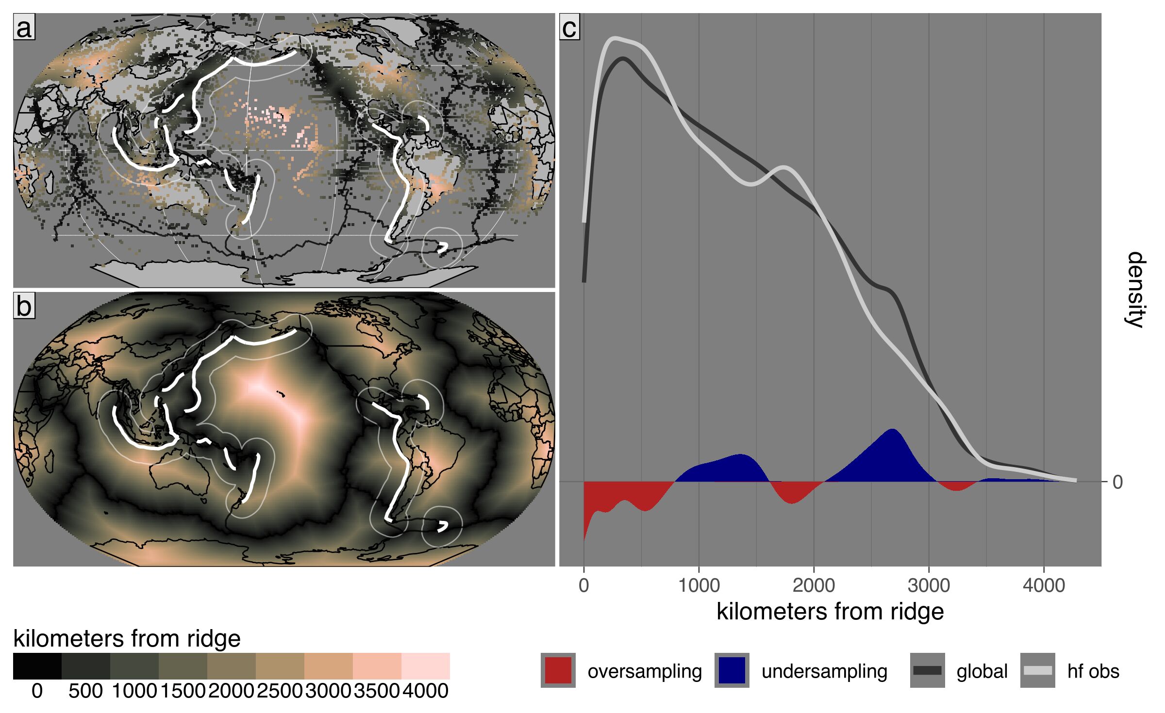
Figure 3.10: Global distribution of surface heat flow observations and distances to ridges. (a, b) Maps showing the localities of surface heat flow observations and their distances from ridges, and the complete global distribution of distances to ridges. (c) Normalized density estimates comparing the relative coverage of surface heat flow observations with the global distribution of distances from ridges. Differences in density reveal regions of over- and undersampling within the geologic proxy parameter space. Subduction zone boundaries (bold white lines) defined by Syracuse & Abers (2006). Plate boundaries defined by Lawver et al. (2018). Global proxy data from Goutorbe et al. (2011).

For Kriging, ideal survey target sites should provide the most regular coverage over a region of interest (e.g. a particular subduction zone segment). Evaluating surface heat flow distributions across upper-plate sectors offers opportunities for discovering future survey targets by identifying the least-constrained sectors. For example, segments with the greatest Similarity-Kriging discrepancies among sectors tend to have: (1) very few ThermoGlobe data (e.g. Alaska Aleutians, N Philippines, New Britain Solomon, S Philippines), (2) highly-irregular spatial coverage of ThermoGlobe data (e.g. Andes, Central America, Lesser Antilles), or (3) complex upper-plate tectonics (Vanuatu). A simple query of the ThermoGlobe dataset by sector can identify individual sectors with low or highly-irregular observational density or large Similarity-Kriging discrepancies. Thus, current observational gaps in regional surface heat flow can be efficiently identified by comparing independent interpolation methods within multiple-sectors.

3.4.3 Comparing Similarity and Kriging Accuracies

Neither error rates nor first principles favor Similarity vs. Kriging on regional (10\(^2\) to 10\(^3\) km) scales. Rather, both methods are successfully generalizable and appropriate for subduction zone research. While some segments do show large discrepancies between Similarity and Kriging error rates (e.g. Scotia), low error rates do not necessarily imply more accurate predictions. For Scotia, few observations naturally lead to overfitting and low error rates, but choosing different Kriging parameters and/or highly localizing Kriging can also unintentionally overfit ThermoGlobe data and compromise regional interpolation accuracy. At 1.3 times greater error rates than Similarity on average, however, Kriging error rates do not suggest overfitting is prevalent (Tables 3.1 and B.1).

Differences in error rates notwithstanding, Similarity has a distinct advantage compared to Kriging when applied to regions with relatively low observational density and/or highly-irregular spatial coverage. For example, Similarity predictions appear to be remarkably consistent with known tectonic features even in cases with few observations (e.g. Scotia and New Britain Solomon, Figures 3.6 & B.11). Integrating geologic proxies is therefore preferred when limited observations preclude practically useful Kriging interpolations.

3.4.4 Layered Interpolation Approach

Similarity and Kriging interpolations are distinguishable by eye at the regional scale (e.g. compare Figures 3.3, 3.5, and 3.6 with the remaining segments in Appendices B.4 & B.5). The same unique properties of Similarity and Kriging methods that make them quickly discernible by eye can be independently leveraged. For example, because Similarity is inherently agnostic to the spatial configuration of observations (Goutorbe et al., 2011), accurate interpolations with well-defined plate boundaries are still possible for regions with relatively few observations (e.g. Scotia and New Britain Solomon, Figures 3.6 & B.11). Since surface heat flow observations near subduction zone segments are commonly sparse and irregularly spaced, spatial-independence from observations is a desirable property to maintain during the interpolation process.

On the other hand, conserving the “ground-truth” is an equally desirable property. Local ordinary Kriging conserves ground-truth by remaining agnostic to all other factors but the spatial configuration of surface heat flow observations (see Appendix B.1). For example, Kriging resolves tectonic features near Tonga New Zealand and Vanuatu that are discordant with Similarity predictions, yet compatible with ThermoGlobe data (Figures B.14 & 3.4). Another example is the young Cocos Plate near Central America where Similarity predicts relatively high heat flow by proximity to two spreading centers and young oceanic plate age, yet observations of anomalously low surface heat flow (e.g. Hutnak et al., 2008) constrain Kriging predictions to low values. Such contrasting predictions imply ThermoGlobe data violate one or more geologic proxy data sets used by Similarity. In other words, Kriging will tend to highlight anomalies (compared to Similarity) if they exist and have been observed.

In principle, carefully layering Similarity and Kriging methods may combine their properties to produce more accurate regional interpolations in the future. A layered approach simultaneously respects the First (Krige, 1951) and Third Laws of Geography (Zhu et al., 2018) by integrating geologic and spatial information. Many methods may be applied to combine Similarity and Kriging predictions. As a basic example: (1) compare Similarity and Kriging layers to detect anomalies, (2) compute weights proportional to the squared difference between Similarity and Kriging predictions to emphasized or subdue anomalies, (3) combine Similarity and Kriging layers using a weighted average scheme.

3.5 Conclusions

This study evaluates regional patterns of surface heat flow near subduction zones by comparing Similarity and Kriging interpolations across adjacent upper-plate sectors. Methodological differences between Similarity and Kriging yield both similar and disparate predicted heat flow distributions and profiles among subduction zones. Four key conclusions arise from regional surface heat flow near active subduction zones:

1. Accurate regional interpolations of irregularly-spaced ThermoGlobe data are key to understanding broad (segment-scale) variations in lithospheric thermal structure near subduction zones.

2. Mixed upper-plate surface heat flow distributions and profiles imply various degrees of regional continuity among subduction zones in terms of their lithospheric thermal structure (contrary to expectations from Kerswell et al., 2021), heat-transferring subsurface dynamics, and/or observational density relative to the local spatial variability of surface heat flow.

3. Future surface heat flow surveys can maximize Similarity and Kriging accuracies by carefully considering the existing spatial distribution of surface heat flow observations and their distribution within geologic proxy parameter space.

4. Layered interpolation approaches may produce more accurate surface heat flow predictions by combining the independently-advantageous properties of Similarity and Kriging methods.

4 Computing Rates and Distributions of Rock Recovery in Subduction Zones

Abstract

Bodies of rock that are detached (recovered) from subducting oceanic plates, and exhumed to Earth’s surface, become invaluable records of the mechanical and chemical processing of rock along subduction interfaces. Exposures of interface rocks with high-pressure (HP) mineral assemblages provide insights into the nature of rock recovery, yet various inconsistencies arise when directly comparing the rock record with numerical simulations of subduction. Constraining recovery rates and depths from the rock record presents a major challenge because small sample sizes of HP rocks reduce statistical power. As an alternative approach, this study implements a classification algorithm to identify rock recovery in numerical simulations of oceanic-continental convergence. Over one million markers are classified from 64 simulations representing a large range of subduction zones. Recovery pressures (depths) correlate strongly with convergence velocity and moderately with oceanic plate age, while slab-top thermal gradients correlate strongly with oceanic plate age and upper-plate thickness. Recovery rates strongly correlate with upper-plate thickness, yet show no correlation with convergence velocity or oceanic plate age. Likewise, pressure-temperature (PT) distributions of recovered markers vary among numerical experiments and generally show deviations from the rock record that cannot be explained by petrologic uncertaineties alone. For example, a significant gap in marker recovery is found near 2 GPa and 550 ˚C, coinciding with the highest frequencies of exhumed HP rocks. Explanations for such a gap in marker recovery include numerical modeling uncertainties, selective sampling of exhumed HP rocks, or natural geodynamic factors not accounted for in numerical experiments.

4.1 Introduction

Maximum pressure-temperature (PT) conditions have been estimated for hundreds of high-pressure (HP) metamorphic rocks exhumed from subduction zones (Figure 4.1, Agard et al., 2018; Hacker, 1996; Penniston-Dorland et al., 2015). These samples represent fragments of oceanic crust, continental crust, seafloor sediments, and upper mantle that have detached from subducting oceanic and continental lithospheres at various depths along the interface between subducting and overriding tectonic plates (referred to as “recovery” after Agard et al., 2018). This rock record is the only tangible evidence of PT-strain fields, deep seismic cycling, and fluid flow within Earth’s lithosphere during deformation and chemical processing in subduction zones. Together with geophysical imaging (e.g., Bostock, 2013; Ferris et al., 2003; Hyndman & Peacock, 2003; Mann et al., 2022; Naif et al., 2015; Rondenay et al., 2008; Syracuse & Abers, 2006), analysis of surface heat flow data (e.g., Currie & Hyndman, 2006; Gao & Wang, 2014; Hyndman et al., 2005; Kohn et al., 2018; Morishige & Kuwatani, 2020; Wada & Wang, 2009), and forward numerical geodynamic modeling (e.g., Gerya et al., 2002, 2008; Gerya & Stöckhert, 2006; Hacker et al., 2003; Kerswell et al., 2021; McKenzie, 1969; Peacock, 1990, 1996; Sizova et al., 2010; Syracuse et al., 2010; Yamato et al., 2007, 2008), investigation of the rock record underpins contemporary understandings of subduction geodynamics (e.g., Agard et al., 2009; Agard, 2021; Bebout, 2007).

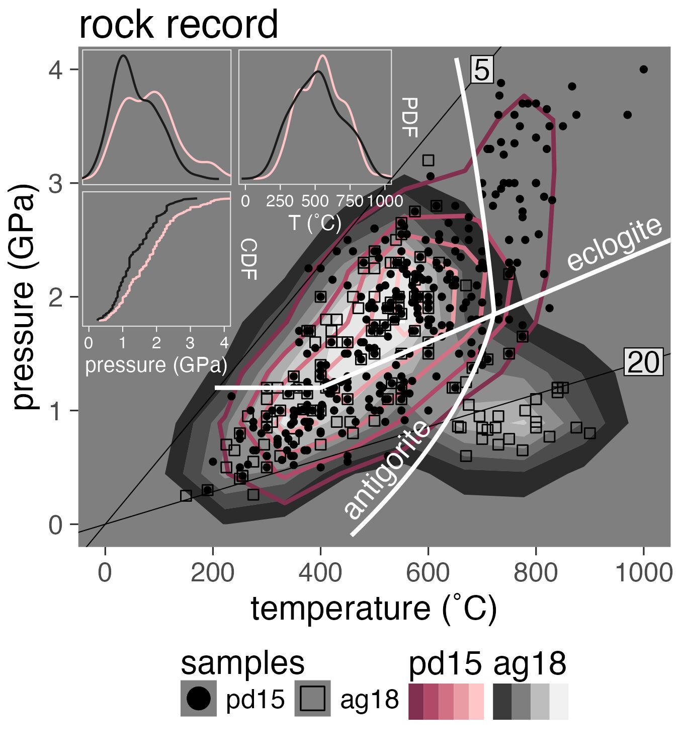
Figure 4.1: PT diagram showing distributions of PT estimates for exhumed HP metamorphic rock samples compiled in the pd15 (solid contours, Penniston-Dorland et al., 2015) and ag18 (filled contours, Agard et al., 2018) datasets. Thin lines are thermal gradients labeled in ˚C/km. Reaction boundaries for eclogitization of oceanic crust and antigorite dehydration are from Ito & Kennedy (1971) and Schmidt & Poli (1998), respectively. (insets) Probability distribution functions of pd15 (pink lines) and ag18 samples (black lines) showing broad bimodal and trimodal sample distributions with respect to P (top left inset) and a kinked CDF (bottom inset) indicating that a substantial proportion of rocks are recovered from P’s between 0.5-2.5 GPa with very few rocks reaching maximum P’s above 3 GPa.

However, it remains difficult to directly interpret the rock record in terms of recovery rates and distributions along the subduction interface. For example, compilations of PT estimates representing the global distribution of HP rocks exhumed during the Phanerozoic (the pd15 and ag18 datasets, Agard et al., 2018; Penniston-Dorland et al., 2015) reveal an abrupt decrease in relative sample abundance at P’s above 2.3-2.4 GPa (Figure 4.1 inset). For pd15 and ag18, a nearly-constant cumulative distribution function (CDF) interrupted by a sharp change in slope around 2.3-2.4 GPa implies relatively widespread recovery of subducting material up to 2.3-2.4 GPa, but increasingly rare recovery at higher P (Agard et al., 2018; Kerswell et al., 2021; Kohn et al., 2018; Monie & Agard, 2009; Plunder et al., 2015). On the one hand, evidence for common mechanical coupling depths near 2.3 GPa (Furukawa, 1993; Kerswell et al., 2021; Wada & Wang, 2009) suggests an upper-limit to recovery depths that is consistent with the scarcity of (ultra-)HP samples in the rock record and invariant with respect to key thermo-kinematic parameters (convergence velocity, subduction geometry, plate thickness; Figure 4.1). On the other hand, geophysical constraints on the depths of key mechanical transitions likely to induce rock recovery (e.g., Abers et al., 2020; Audet & Kim, 2016; Audet & Schaeffer, 2018; Morishige & Kuwatani, 2020) suggest high recovery rates should cluster around discrete depths, rather than widespread recovery along the subduction interface implied by the pd15 and ag18 datasets.

Difficulties in relating complex polymetamorphic rocks from different environments challenge the use of PT distributions of exhumed HP rock samples as robust constraints on key subduction zone parameters. Interpretations of rock recovery mechanisms, subduction interface behavior, metamorphic reactions, seismic cycling, and subduction geodynamics might vary depending on metamorphic terrane (local tectonic environment), sampling strategy (random or targeted outcrops), sample size (how many outcrops were observed and sampled in the field), and analytical sample selection (investigating PTs and deformation histories for a subset of samples with a specific scientific question in mind). Different compilations of PT estimates from natural samples can show different distributions in terms of relative abundances (frequencies) of samples across PT space, and thus imply a natural preference of rock recovery (and/or exhumation) from different depths along the subduction interface. For example, Agard et al. (2018) noted that compilations from Plunder et al. (2015) and Groppo et al. (2016) show less dispersion (i.e., a more step-like CDF) than ag18 with tighter bimodal or trimodal distributions clustering around inferred depths of important mechanical transitions along the subduction interface. That is, high-frequency peaks (modes) in PT distributions of exhumed HP rocks are inferred to coincide with the continental Moho at approximately 25-35 km and the transition to mechanical plate coupling at approximately 80 km (Agard et al., 2018; Monie & Agard, 2009; Plunder et al., 2015). Less attention in the literature is paid to a smaller, yet significant, intermediate mode at 55-60 km (Agard et al., 2009, 2018; Plunder et al., 2015), although it is consistent with a high-frequency region of PT estimates in the pd15 dataset.

Differences in compiled PT datasets notwithstanding, key observations regarding rock recovery in subduction zones emerge from pd15 and ag18:

Pressure

• Rock recovery is broadly and unequally distributed
• Rock recovery is more frequent near 1 GPa and 2 GPa (bimodal)
• 64-66% of recovered rocks equilibrated between 1-2.5 GPa
• 5-19% of recovered rocks equilibrated above 2.5 GPa

Temperature

• 50-56% of recovered rocks equilibrated above 525 ˚C
• 32-34% of recovered rocks equilibrated between 350-525 ˚C

PT gradient

• 52-62% of recovered rocks record gradients between 5-10 ˚C/km
• 18-31% of recovered rocks record gradients between 10-15 ˚C/km
• 6-30% of recovered rocks record gradients above 15 ˚C/km

These ranges in the relative abundances of exhumed HP rocks compiled in different datasets raise important questions in subduction zone research: are rocks recovered broadly and uniformly along the subduction interface or discretely from certain depths? How do recovery rates and distributions vary among diverse subduction zone settings and through time?

Previous work comparing the rock record directly with numerical models has generally produced ambiguous interpretations concerning recovery rates (the volumetric ratio of recovered:subducted material) and PT distributions of recovery along the subduction interface—especially with respect to P, or depth. For example, comparisons of different numerical geodynamic codes with subsets of the rock record show variable agreement in terms of overlapping PT paths and thermal gradients (e.g., Angiboust et al., 2012b; Burov et al., 2014; Holt & Condit, 2021; Penniston-Dorland et al., 2015; Plunder et al., 2018; Roda et al., 2010, 2012, 2020; Ruh et al., 2015; Yamato et al., 2007, 2008). Numerous factors potentially contribute to inconsistent PT distributions and thermal gradients between exhumed HP rocks and numerical geodynamic models, including initial setups for numerical experiments and ranges in thermo-kinematic boundary conditions (i.e., subduction zone setting: oceanic plate age, convergence velocity, subduction dip angle, upper-plate thickness, and heating sources; Kohn et al., 2018; Penniston-Dorland et al., 2015; Ruh et al., 2015; van Keken et al., 2019), differential recovery rates from subduction zones with favorable settings (Abers et al., 2017; van Keken et al., 2018), and comparisons among suites of undifferentiated HP rocks (e.g., grouping rocks recovered during subduction initiation with rocks recovered during “steady-state” subduction, see Agard et al., 2018, 2020). Compounding the ambiguity are arguments that material is sporadically recovered during short-lived mechanical transitions (Agard et al., 2016) and/or geodynamic changes (Monie & Agard, 2009)—implying exhumed HP rocks are not random samples of the subduction interface during steady-state subduction. Such ambiguities warrant further investigation into the general response of recovery rates and distributions to broad ranges of subduction zone settings and various implementations of subduction interface rheologies.

Fortunately, clues about the nature and PT limits of rock recovery are provided by many extensively studied examples of exhumed subduction interfaces (e.g., Agard et al., 2018; Angiboust et al., 2011, 2015; Cloos & Shreve, 1988; Fisher et al., 2021; Ioannidi et al., 2020; Kitamura & Kimura, 2012; Kotowski & Behr, 2019; Locatelli et al., 2019; Monie & Agard, 2009; Okay, 1989; Platt, 1986; Plunder et al., 2013, 2015; Tewksbury-Christle et al., 2021; Wakabayashi, 2015). However, these type localities represent an unknown fraction of subducted material and differ significantly in terms of their geometry (field relationships), composition (rock types), and interpreted deformation histories (both detachment and exhumation). It is also unclear to what extent ag18 and pd15 (and other compilations) represent the full range of recovery conditions and/or represent scientific sampling bias (e.g., undersampling low-grade rocks or oversampling high-grade rocks from the same pristine exposures, Agard et al., 2018) or other geodynamic biases (e.g., preferential exhumation, Abers et al., 2017; van Keken et al., 2018). Thus, a primary challenge to inferring recovery rates and distributions accurately from the rock record fundamentally stems from sparse nonrandom samples (typically less than a few dozen PT estimates from any given exhumed terrane) compared to the diversity of thermo-kinematic parameters characterizing subduction zones and dynamic petro-thermo-mechanical processes that might trigger rock recovery along the subduction interface.

This study aims at addressing the sparsity and nonrandomness of exhumed HP rock samples by tracing numerous (1,341,729) Lagrangian markers from 64 numerical geodynamic simulations of oceanic-continental subduction (Kerswell et al., 2021). We first generate a PT dataset from instantiations of a particular numerical geodynamic code so large that it was insensitive to noise and outliers—thus representing a statistically robust picture of recovery rates and PT distributions of recovery in subduction zone models. From such a large dataset of generated samples, we identify correlations among recovery rates, PT distributions, and subduction zone settings (i.e., oceanic plate age, convergence velocity, and upper-plate thickness) that test sensitivities and indicate ranges of plausible conditions for reproducing the rock record. In fact, numerical experiments predict surprisingly few recovered samples corresponding with the PT region around 2 GPa and 550 ˚C—the same PT region that has a relatively high-frequency of natural samples. We then discuss implications for inconsistencies between frequencies of generated samples and exhumed HP rocks, including insufficient implementation of recovery mechanisms in numerical geodynamic models (numerical bias), a potential overabundance of natural samples collected from similar metamorphic grades around 2 GPa and 550 ˚C (sampling bias), and preferential exhumation from a relatively narrow range of PT conditions (geodynamic bias).

4.2 Methods

This study presents a dataset of Lagrangian markers (described below) from numerical experiments that simulated 64 oceanic-continental convergent margins with thermo-kinematic boundary conditions (oceanic plate age, convergence velocity, and upper-plate lithospheric thickness) closely representing the range of presently active subduction zone settings (Syracuse & Abers, 2006; Wada & Wang, 2009). Initial conditions were modified from previous studies of active margins (Gorczyk et al., 2007; Sizova et al., 2010) using the numerical geodynamic code I2VIS (Gerya & Yuen, 2003), which models visco-plastic flow of geological materials by solving conservative equations of mass, energy, and momentum on a fully-staggered finite difference grid with a marker-in-cell technique (e.g., Gerya, 2019; Gerya & Yuen, 2003; Harlow & Welch, 1965). Complete details about the initial setup, boundary conditions, and rheological model are presented in Kerswell et al. (2021). Complete details about I2VIS and example code are presented in Gerya & Yuen (2003) and Gerya (2019).

The following section summarizes the numerical modeling setup, then defines Lagrangian markers (now referred to as markers) and briefly elaborates on their usefulness in understanding flow of geological materials, followed finally by a description of the marker classification algorithm. A complete mathematical description of the classification algorithm is presented in Appendix C.1.

4.2.1 Summary of the Numerical Modeling Setup

The numerical geodynamic models of Kerswell et al. (2021) used for generating the markers dataset in this study are 2000 km wide and 300 km deep with nonuniform resolution that increases gradually from 5 \(\times\) 1 km at the boundaries (in the x- and z-directions, respectively) to 1 \(\times\) 1 km within a 600 km wide area surrounding the contact between the oceanic plate and continental margin. The left and right boundaries are free-slip and thermally insulating. “Sticky” air and water at the top boundary allow for a free topographical surface with a simple linear implementation of sedimentation and erosion. The lower boundary is open to allow for free subduction geometries during oceanic plate descent (Burg & Gerya, 2005).

4.2.1.1 Rheological Model

All rock types within the model domain are treated as visco-plastic materials by limiting diffusion and dislocation creep deformation mechanisms with a brittle (plastic) yield criterion. Contributions from dislocation and diffusion creep are accounted for by computing a composite rheology for ductile rocks, \(\eta_{eff}\): \[\begin{equation} \begin{aligned} \frac{1}{\eta_{eff}} = \frac{1}{\eta_{diff}} + \frac{1}{\eta_{disl}} \end{aligned} \tag{2.1} \end{equation}\] where \(\eta_{diff}\) and \(\eta_{disl}\) are effective viscosities for diffusion and dislocation creep.

For the crust and serpentinized mantle, \(\eta_{diff}\) and \(\eta_{disl}\) are computed as: \[\begin{equation} \begin{aligned} \eta_{diff} &= \frac{1}{2} \ A \ \sigma_{crit}^{1-n} \ \exp\left[\frac{E+PV}{RT}\right] \\ \eta_{disl} &= \frac{1}{2} \ A^{1/n} \ \dot{\varepsilon}_{II}^{(1-n)/n} \ \exp\left[\frac{E+PV}{nRT}\right] \end{aligned} \tag{2.2} \end{equation}\] where \(R\) is the gas constant, \(P\) is pressure, \(T\) is temperature in \(K\), \({\dot{\varepsilon}}_{II} = \sqrt{\frac{1}{2}{{\dot{\varepsilon}}_{ij}}^{2}}\) is the square root of the second invariant of the strain rate tensor, \(\sigma_{crit}\) is an assumed diffusion-dislocation transition stress, and \(A\), \(E\), \(V\) and \(n\) are the material constant, activation energy, activation volume, and stress exponent, respectively (Table 4.1, Hilairet et al., 2007; Ranalli, 1995).

For the mantle, \(\eta_{diff}\) and \(\eta_{disl}\) are computed as (Karato & Wu, 1993): \[\begin{equation} \begin{aligned} \eta_{diff} &= \frac{1}{2} \ A^{-1} \ G \ \left[\frac{h}{b}\right]^{m/n} \ \exp\left[\frac{E+PV}{RT}\right] \\ \eta_{disl} &= \frac{1}{2} \ A^{-1/n} \ G \ \dot{\varepsilon}_{II}^{(1-n)/n} \ \exp\left[\frac{E+PV}{nRT}\right] \end{aligned} \tag{2.3} \end{equation}\] where \(b\) = 5 \(\times\) 10\(^{-10}\) m is the Burgers vector, \(G\) = 8 \(\times\) 10\(^{10}\) Pa is shear modulus, \(h\) = 1 \(\times\) 10\(^{-3}\) m is the assumed grain size, \(m\) = 2.5 is the grain size exponent, and the other flow law parameters are given in Table 4.1. Viscosity is limited in all numerical experiments from \(\eta_{min}\) = 10\(^{17}\) Pa \(\cdot\) s to \(\eta_{max}\) = 10\(^{25}\) Pa \(\cdot\) s.

An effective visco-plastic rheology is achieved by limiting \(\eta_{eff}\) with a brittle (plastic) yield criterion: \[\begin{equation} \eta_{eff} \leq \frac{C + \phi \ P}{2 \ \dot{\varepsilon}_{II}} \tag{2.4} \end{equation}\] where \(\phi\) is the internal friction coefficient, \(C\) cohesive strength at \(P\) = 0, and \({\dot{\varepsilon}}_{ij}\) is the strain rate tensor (Table 4.1).

Table 4.1: Material properties used in numerical experiments

Material	\(\rho\)	\(H_2O\)	Flow Law	\(log_{10}A\)	\(E\)	\(V\)	\(n\)	\(\phi\)	\(\sigma_{crit}\)	\(k_1\)	\(k_2\)	\(k_3\)	\(H\)
	kg/m\(^3\)	\(wt.\%\)			kJ/mol	J/MPa\(\cdot\)mol			MPa				\(\mu\)W/m\(^3\)
sediments	2600	5.0	wet quartzite	-3.5	154.0	3.0	2.3	0.15	0.03	0.64	807	4e-06	2.000
felsic crust	2700		wet quartzite	-3.5	154.0	3.0	2.3	0.45	0.03	0.64	807	4e-06	1.000
basalt	3000	5.0	plag an75	-3.5	238.0	8.0	3.2	0.45	0.03	1.18	474	4e-06	0.250
gabbro	3000		plag an75	-3.5	238.0	8.0	3.2	0.45	0.03	1.18	474	4e-06	0.250
mantle dry	3300		dry olivine	4.4	540.0	20.0	3.5	0.45	0.30	0.73	1293	4e-06	0.022
mantle hydrated	3300	0.5	wet olivine	3.3	430.0	10.0	3.0	0.45	0.24	0.73	1293	4e-06	0.022
serpentine	3200	2.0	serpentine	3.3	8.9	3.2	3.8	0.15	3.00	0.73	1293	4e-06	0.022
key: \(A\): material constant, \(E\), \(V\): activation energy and volume, \(n\): power law exponent, \(\phi\): internal friction angle, \(\sigma_{crit}\): critical stress, \(k_1\)-\(k_3\): thermal conductivity constants, \(H\): heat production
constants: \(C_p\): heat capacity = 1 [kJ/kg], \(\alpha\): expansivity = 2\(\times 10^{-5}\) [1/K], \(\beta\): compressibility = 0.045 [1/MPa]
thermal conductivity: \(k\) [W/mK] = \((k_1+\frac{k_2}{T+77})\times exp(k_3 \cdot P)\) with \(P\) in [MPa] and \(T\) in [K]
references: Turcotte & Schubert (2002), Ranalli (1995), Hilairet et al. (2007), Karato & Wu (1993)

4.2.1.2 Metamorphic (De)Hydration Reactions

Within the model domain, free water particles are generated and consumed by empirically-derived (de)hydration reactions and migrate with relative velocities defined by local deviatoric (non-lithostatic) pressure gradients (Faccenda et al., 2009). In the subducting lithosphere, gradual eclogitization of oceanic crust is computed as a linear function of lithostatic pressure. This effectively simulates continuous influx of water to the upper-plate mantle beginning with compaction and release of connate water at shallow depths, followed by a sequence of reactions consuming major hydrous phases (chlorite, lawsonite, zoisite, chloritoid, talc, amphibole, and phengite) in different parts of the hydrated basaltic crust (Schmidt & Poli, 1998; van Keken et al., 2011). Besides gradual water release, eclogitization of the oceanic crust involves densification at the garnet-in and plagioclase-out reaction boundaries defined by Ito & Kennedy (1971).

In the upper-plate mantle wedge, formation of brucite and serpentine from dry olivine is inferred to strongly regulate mechanical behavior of the plate interface (Agard et al., 2016; Hyndman & Peacock, 2003; Peacock & Hyndman, 1999). Because brucite breaks down at much lower temperatures than serpentine (e.g., Bowen & Tuttle, 1949; Schmidt & Poli, 1998), serpentine (de)stabilization is arguably more responsible for regulating interface rheology deep in subduction zones. Thus, Kerswell et al. (2021) chose to explicitly model serpentine (de)hydration in the upper mantle, which effectively induces a mechanical (de)coupling transition at the \(antigorite \Leftrightarrow olivine + orthopyroxene + H_{2}O\) reaction boundary defined by Schmidt & Poli (1998). All such (de)hydration reactions tacitly assume thermodynamic equilibrium.

4.2.2 Lagrangian Markers

Markers are mathematical objects representing discrete parcels of material flowing in a continuum (Harlow, 1962, 1964). Tracing markers (saving marker information at each timestep) advances the investigation of subduction dynamics in the following two ways.

First, modeling subduction requires solving equations of mass, motion, and heat transport in a partly layered, partly heterogeneous, high-strain region known as the plate interface, subduction interface, or subduction channel (Gerya et al., 2002). Current conceptual models regard the subduction interface as a visco-plastic continuum with complex geometry and structure, sharp thermal, chemical, and strain gradients, strong advection, and abundant fluid flow (Agard et al., 2016, 2018; Bebout, 2007; Bebout & Barton, 2002; Cloos & Shreve, 1988; Gerya & Yuen, 2003; Shreve & Cloos, 1986; Stöckhert, 2002; Tewksbury-Christle et al., 2021). Finite-difference numerical approaches do not perform well with strong local gradients, and interpolating and updating T, strain, and chemical fields with markers greatly improves accuracy and stability of numerical solutions (Gerya, 2019; Gerya & Yuen, 2003; Moresi et al., 2003).

Second, tracing a marker closely proxies for tracing a rock’s PT-time history. Strictly speaking, deviations between calculated PT-time histories of markers and rocks are possible because the numerical geodynamic simulations assume: (1) markers move in an incompressible continuum (Batchelor, 1953; Boussinesq, 1897), (2) material properties are governed by a simplified petrologic model describing eclogitization of oceanic crust (Ito & Kennedy, 1971) and (de)hydration of upper mantle (\(antigorite \Leftrightarrow olivine + orthopyroxene + H_{2}O\), Schmidt & Poli, 1998), and (3) marker stress and strain are related by a highly non-linear rheological model derived from empirical flow laws (Hilairet et al., 2007; Karato & Wu, 1993; Ranalli, 1995; Turcotte & Schubert, 2002). For example, if rocks within a subduction interface shear zone were highly compressible or could sustain large deviatoric stresses, P’s and T’s might be different from markers.

The rheological model implemented in the numerical simulations of Kerswell et al. (2021), embodied by assumptions 2 and 3, exert particularly strong control on subduction interface strength, and thus the probability and style of detachment. For example, all numerical simulations from Kerswell et al. (2021) developed stable subduction channels (tectonic-mélanges, e.g., Gerya et al., 2002) instead of discrete shear zones that detach large coherent slices of oceanic lithosphere (e.g., Ruh et al., 2015) primarily due to the choice of rheological model and specific implementation of metamorphic (de)hydration reactions. A major uncertainty in the markers dataset presented below stems from an implicit assumption that the plate interface behaves like a distributed shear zone composed of hydrated ultramafic material mixed with fragments of dehydrating oceanic crust and seafloor sediments (i.e., a tectonic mélange). Field evidence for tectonic slicing of HP rocks does not necessarily support this view of plate interface behavior (e.g., Agard et al., 2018; Angiboust et al., 2009, 2012a, 2014b; Gilio et al., 2020; Locatelli et al., 2018; Monie & Agard, 2009; Poulaki et al., 2023), while other well-studied mélange-like structures do (e.g., Festa et al., 2019; Harvey et al., 2021; Hsü, 1968; Kusky et al., 2013; Penniston-Dorland & Harvey, 2023; Platt, 2015; Wakabayashi & Dilek, 2011), and still other localities exhibit field relations that are more ambiguous (e.g., Bonnet et al., 2018; Cisneros et al., 2022; Kotowski et al., 2022; Kusky et al., 2013; Platt, 1975). Such a variety of different structures interpreted as former plate interfaces highlight the fact that large uncertainties exist in the rock record—in addition to large experimental and theoretical uncertainties—all of which challenge our understanding of plate interface mechanics in subduction zones. Large uncertainties notwithstanding, our objective was to assess the rates and PT distribution of HP rock recovery during steady state subduction in a distributed shear zone, not necessarily during short-lived events that might induce tectonic slicing of subducting lithosphere. Therefore, insofar as the plate interface approximates a mélange-like channel of incompressible visco-plastic fluid (under the assumptions above, Gerya, 2019; Gerya & Yuen, 2003; Kerswell et al., 2021), first-order comparisons between marker PT distributions and the rock record may be made.

4.2.3 Marker Classification

For each numerical experiment, 20,986 markers were initially selected from within a 760 km-long and 8 km-deep section of oceanic crust and seafloor sediments at \(t\) = 0 Ma. Tracing proceeded for 115 timesteps (between 9.3-54.7 Ma depending on convergence velocity), which was sufficient for markers to be potentially subducted very deeply (up to 300 km) from their initial positions. To a first-order, however, only markers that detached from the subducting oceanic plate (i.e., not subducted) were relevant for comparison with PT estimates of exhumed HP rocks. The main challenge, therefore, was to first develop a method for determining which markers among 20,986 detached from the subducting plate without knowing their fate a priori. Moreover, the method needed to be generalizable to a large range of numerical experiments.

Classifying unlabelled markers as either “recovered” or “not recovered” based solely on their undifferentiated traced histories defines an unsupervised classification problem (Barlow, 1989). Many methods can be applied to solve the unsupervised classification problem, yet this study implemented a Gaussian mixture model (Reynolds, 2009)—a type of “soft” clustering algorithm used extensively for pattern recognition, anomaly detection, and estimating complex probability distribution functions (e.g., Banfield & Raftery, 1993; Celeux & Govaert, 1995; Figueiredo & Jain, 2002; Fraley & Raftery, 2002; Vermeesch, 2018). “Hard” classification is possible by directly applying simple rules to markers without clustering (e.g., Roda et al., 2012). However, “hard” methods are less generalizable than “soft” approaches like Gaussian mixture models, which can be implemented to study many possible features in numerical simulations with Lagrangian reference frames—not just recovery of subducted material. In this case, a Gaussian mixture model organized markers into groups (clusters) by fitting \(k\) = 14 bivariate Gaussian ellipsoids to the distribution of markers in PT space. “Fitting” refers to adjusting parameters (centroids and covariance matrices) of all \(k\) Gaussian ellipsoids until the ellipsoids and data achieved maximum likelihood (see Appendix C.1 for a complete mathematical description). Finally, marker clusters with centroids located within certain bounds were classified as “recovered”. The entire classification algorithm can be summarized as follows:

Marker classification algorithm

0. Select markers within a 760 km \(\times\) 8 km section of oceanic crust
1. Trace markers for 115 timesteps
2. Identify maximum marker PT conditions (at [maxP, T] or “maxP”)
3. Apply Gaussian mixture modeling to maximum marker PT conditions
4. Check for cluster centroids within the bounds:
   • ≥ 3 ˚C/km AND
   • ≤ 1300 ˚C AND
   • ≤ 120 km (3.4 GPa)
5. Classify marker clusters found in step 4 as “recovered”
6. Classify all other markers as “not recovered”

Note that marker PTs used for clustering were assessed before markers melted. Melting was implemented in the numerical experiments of Kerswell et al. (2021) but was irrelevant for marker clustering. Marker PTs used for clustering were also assessed before the accretionary wedge toe collided with the high-viscosity convergence region positioned at 500 km from the left boundary to avoid spurious PT conditions associated with sudden isothermal burial. We also tested different prograde PT path positions in step 2 by determining maximum marker T’s (P, maxT or “maxT”) and maximum P’s (maxP, T or “maxP”) independently. Applying maxP vs. maxT conditions to the classifier resulted in distinct PT distributions of recovered markers and correlations with subduction zone settings. However, compilations of exhumed HP rocks emphasize maxP, not maxT, (Penniston-Dorland et al., 2015), and thus empirical PT estimates are best compared with maxP conditions. Also, many PT paths for exhumed HP rocks have “hairpin” or isothermal decompression retrograde PT paths without significant heating during exhumation (Agard et al., 2009). Figures 4.2 and 4.3 illustrate marker classification for 1 of 64 numerical experiments. All other experiments are presented in the Appendix C.3.

When evaluating the comparisons between markers and rocks made below, it is important that detached markers classified as “recovered” were not exhumed to the surface within the modeling domain. In fact, very few markers exhumed to any significant degree after detachment from the subducting plate. In natural systems, diverse processes drive exhumation of subduction zone rocks, including later tectonic events (Agard et al., 2009). However, our goal was to compare only the maximum metamorphic conditions of markers and rocks along their prograde paths during steady-state subduction. Because most rocks in pd15 and ag18 are inferred to have relatively tight closed-loop PT paths (Agard et al., 2018; Penniston-Dorland et al., 2015), it is reasonable to assume that their maximum PT estimates closely correspond to the point of detachment (recovery) along the plate interface. Therefore, our analysis compared maximum PT estimates for exhumed rocks with PT conditions during marker detachment from the subducting plate.

4.2.4 Recovery Modes

To better quantify how rock recovery can vary among different subduction zone settings, marker recovery modes (high-frequency peaks) were determined with respect to absolute PT and PT gradients. The highest-frequency peak (mode1) shows where the greatest abundance of markers are recovered. The deepest, or warmest, frequency peak (mode2) shows where the most deeply subducted markers (or markers with the highest PT gradients) are recovered. It is crucial to understand that mode2 represents a very small number of recovered markers compared to mode1 in all cases (typically \(\leq\) 1–10%). In other words, changes in the positions of mode1 and mode2 reflect variations in recovery conditions (P, T, and PT gradients) for “normal” recovery and “extreme cases”, respectively.

Note that correlations are not presented here with respect to the thermal parameter \(\Phi\) (\(\Phi\) = oceanic plate age \(\cdot\) convergence velocity), unlike other studies (e.g., England et al., 2004; Wada & Wang, 2009). The rationale is three-fold: (1) the aim was to understand how oceanic plate age and convergence velocity affect marker recovery independently, (2) sample sizes of recovered markers were larger when grouped by oceanic plate age and convergence velocity (n = 335,788) compared to grouping by \(\Phi\) (n = 83,947; implying they do not correlate well with \(\Phi\)), and (3) combining oceanic plate age and convergence velocity can draw unnecessarily ambiguous associations with other geodynamic features of subduction zones (e.g., \(\Phi\) vs. \(H\) from England et al., 2004; Wada & Wang, 2009).

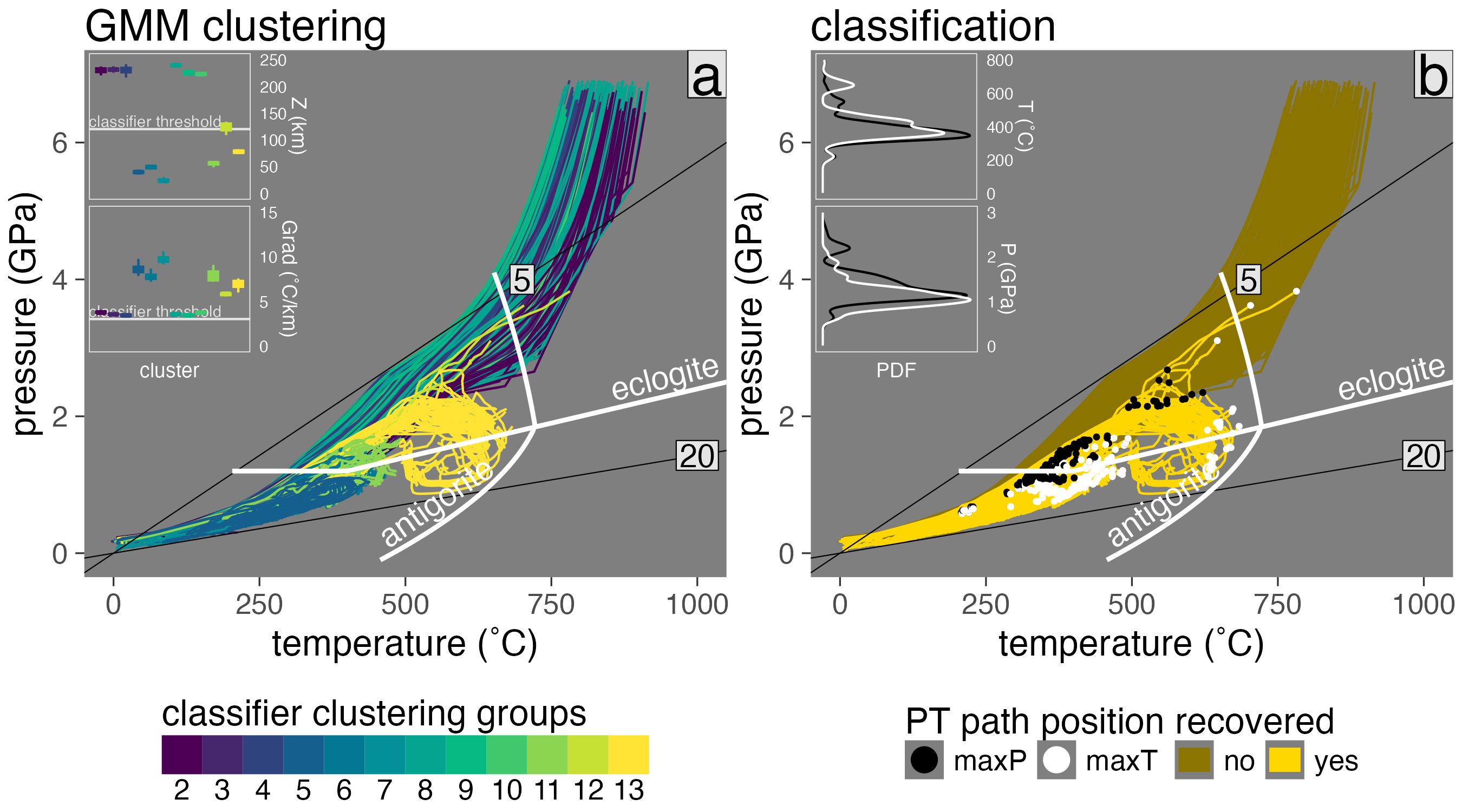
Figure 4.2: Example of marker classification for model cda62. (a) PT diagram showing marker clusters as assigned by Gaussian mixture modeling (GMM; colored PT paths). Boxplots showing depth and thermal gradient distributions of marker clusters assigned by GMM. Markers belonging to clusters with centroids (means) positioned at ≤ 120 km (top inset) and ≥ 3 ˚C/km (bottom inset) are classified as recovered. All others are classified as not recovered. (b) PT diagram showing marker classification results (colored PT paths) and various marker positions along their PT paths (black, white, and pink points). Thin lines are thermal gradients labeled in ˚C/km. Only a random subset of markers is shown. (insets) Probability distribution functions showing the distribution of T’s (top inset) and P’s (bottom inset) for recovered markers at maxP (black lines) and maxT (white lines) conditions. In this experiment, a significant number of markers have different peak metamorphic conditions between their maxT and maxP positions.

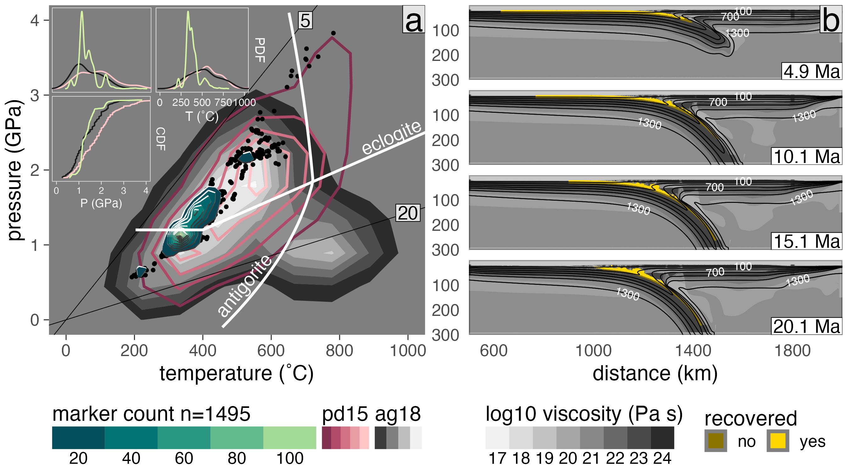
Figure 4.3: Summary of marker recovery for model cda62. (a) PT diagram showing the frequency of recovered markers (black points and green Tanaka contours) in comparison with the pd15 (solid red contours) and ag18 (filled gray contours) datasets. Thin lines are thermal gradients labeled in ˚C/km. Reaction boundaries for eclogitization of oceanic crust and antigorite dehydration are from Ito & Kennedy (1971) and Schmidt & Poli (1998), respectively. Marker counts (Tanaka contours) are computed across a 100 \(\times\) 100 grid (0.04 GPa \(\times\) 10 ˚C). (insets) Probability distribution functions (top insets) and cumulative distribution functions (bottom inset) comparing P and T distributions between numerical experiments (green lines) and natural samples (pink lines: pd15, black lines: ag18). (b) Visualization of log viscosity in the model domain showing the major modes of marker recovery along a relatively thick subduction interface that tapers near the viscous coupling depth.

4.3 Results

4.3.1 Markers vs. the Rock Record

4.3.1.1 Markers from all Numerical Experiments

While marker recovery can occur at all P’s recorded by exhumed metamorphic rocks (Figure 4.4), numerical experiments predict that most markers are recovered from discrete regions (depths) along the plate interface. For example, pd15 and ag18 show high sample frequencies from near 1 GPa—a shared feature common to all 64 numerical experiments. Yet samples recovered from above 1 GPa are much more frequent in pd15 and ag18 compared to simulations (relative to the total number of samples in each dataset; Figure 4.4 inset). Samples compiled in pd15 and ag18 also show much broader bimodal or trimodal distributions across P’s compared to a narrow unimodal P distribution centered at 1 GPa for recovered markers.

With respect to T, thermal gradients of recovered markers are significantly lower than natural samples. On average, markers recovered from < 2 GPa differ from rocks exhumed from < 2 GPa by 173 ˚C and 3-4 ˚C/km (excluding the highest-T samples in ag18 that relate to subduction initiation, Agard et al., 2018, 2020; Soret et al., 2022). Even within typical uncertainties for thermobarometry and phase equilibrium modeling (c. ± 0.1–0.15 GPa and ± 50 ˚C, Kohn & Spear, 1991; Penniston-Dorland et al., 2015; Spear, 1993), major discrepancies exist between the high-frequency peak of recovered markers centered at 1 GPa and 275˚ C and the high-frequency peaks of natural samples centered at 1 GPa and 380˚ C and 2 GPa and 550˚ C (compare Figures 4.1 and 4.4). However, when comparing the distribution of samples around 1 GPa, rather than modal peak positions, moderate overlap does exist between T’s of markers and natural samples.

4.3.1.2 Markers from Individual Numerical Experiments

For most experiments, marker recovery is localized within discrete and narrow multimodal distributions with step-like CDFs [e.g., 4.3]. The PT positions of recovery clusters vary with subduction zone setting, however, so comparisons between individual numerical experiments and the rock record are challenging. For example, a few experiments show broad marker distributions that resemble the rock record with respect to P, but not with respect to thermal gradients (Appendix C.3). Other experiments show the opposite. To better compare marker recovery among various subduction zone settings, we combined recovered markers from multiple numerical experiments with similar thermo-kinematic boundary conditions—analogous to randomly sampling exhumed HP rocks from similar subduction zones (Figures 4.5 and 4.6).

Whether comparing the rock record with recovered markers from individual numerical experiments, suites of experiments, or all numerical experiments, several key observations emerge:

1. Recovered markers from most individual numerical experiments show discrete multimodal PT distributions with steep step-like CDFs (Figure 4.3 and Appendix C.3)
2. While relatively few markers are recovered from PT regions coinciding with high-frequencies of natural samples around 2 GPa and 550 ˚C, markers and natural samples recovered from near 1 GPa show moderate overlap (compare Figures 4.4, 4.5, and 4.6)
3. Markers are frequently recovered from a major P mode near 1 GPa and very infrequently recovered between 2–2.5 GPa with a higher rate of recovery from lower P’s (79% from ≤ 1.5 GPa) compared to natural samples (36-59% from ≤ 1.5 GPa; compare Figures 4.4, 4.5, and 4.6)
4. Markers are frequently recovered from a major T mode near 275 ˚C and very infrequently recovered between 400–600 ˚C with a higher rate of recovery from lower T’s (97% from ≤ 525 ˚C) compared to natural samples (44-50% from ≤ 525 ˚C; compare Figures 4.4, 4.5, and 4.6)
5. The relative abundance of markers recovered along cooler thermal gradients for subduction zones (87% from 5-12 ˚C/km) is high compared to natural samples (59-78% from 5-12 ˚C/km; compare Figures 4.4, 4.5, and 4.6)
6. Many markers are recovered from the forbidden zone (11% from ≤ 5 ˚C/km; compare Figures 4.4, 4.5, and 4.6)
7. Virtually no markers (0.001%) are recovered from ≥ 15 ˚C/km compared to natural samples (6-30% from ≥ 15 ˚C/km; compare Figures 4.4, 4.5, and 4.6)

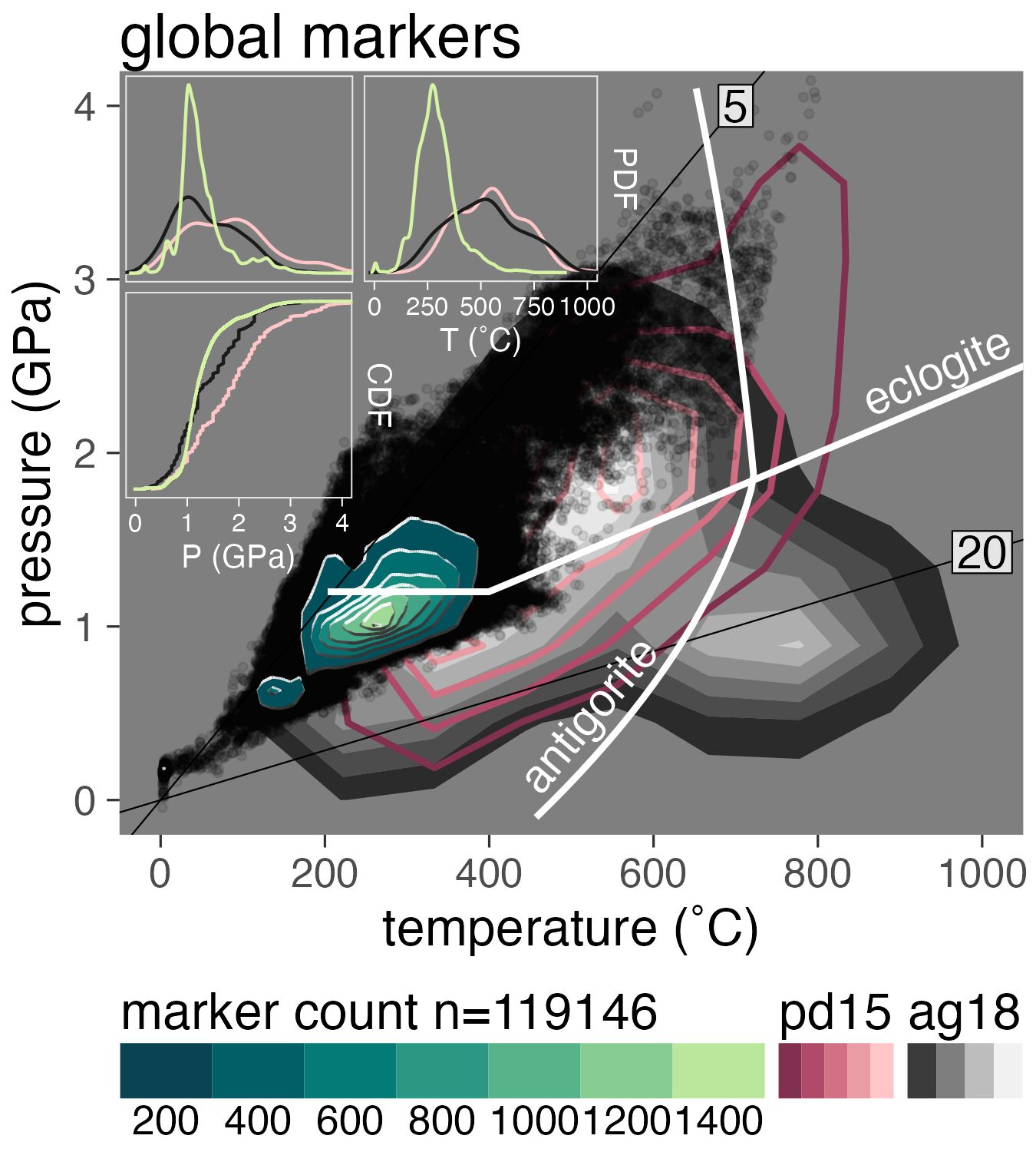
Figure 4.4: PT diagram showing the PT conditions of recovered markers (black point cloud) from all 64 numerical experiments and the frequency of recovered markers (green Tanaka contours) in comparison with the pd15 (solid red contours) and ag18 (filled gray contours) datasets. Marker frequency is concentrated along relatively cool thermal gradients, primarily near the continental Moho (1 GPa), with minor recovery modes centered near the onset of plate coupling (2.3-2.5 GPa). Thin lines are thermal gradients labeled in ˚C/km. Reaction boundaries for eclogitization of oceanic crust and antigorite dehydration are from Ito & Kennedy (1971) and Schmidt & Poli (1998), respectively. Marker counts (Tanaka contours) are computed across a 100 \(\times\) 100 grid (0.04 GPa \(\times\) 10 ˚C). (insets) Probability distribution functions (top insets) and cumulative distribution functions (bottom inset) comparing P and T distributions between numerical experiments (green lines) and natural samples (pink lines: pd15, black lines: ag18). Note the higher-abundance of pd15 and ag18 samples at P > 1.5 GPa compared to markers.

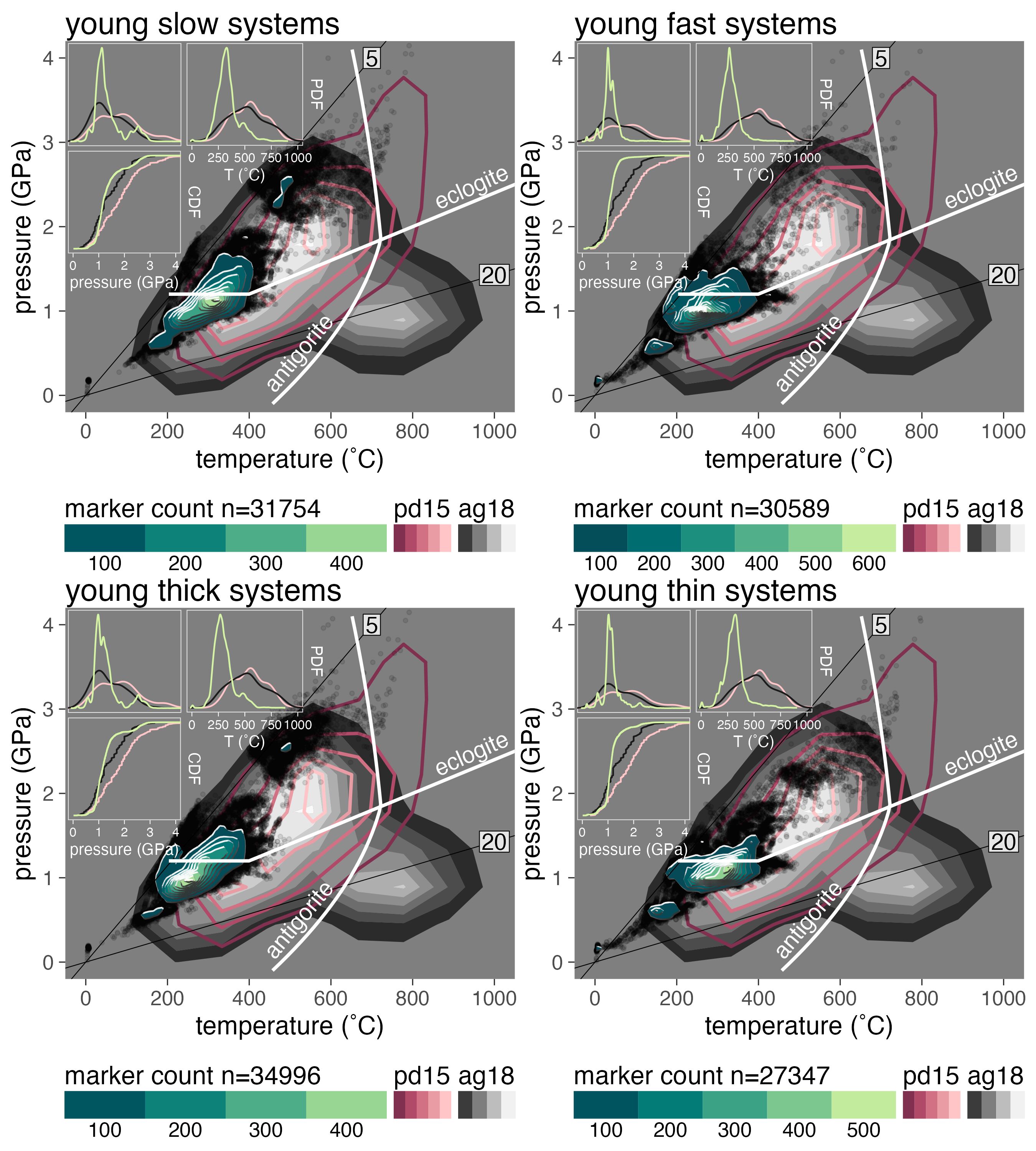
Figure 4.5: PT diagram showing the PT conditions of recovered markers (black point clouds) from numerical experiments with young oceanic plates (32.6-55 Ma) and the frequencies of recovered markers (green Tanaka contours) in comparison with the pd15 (solid red contours) and ag18 (filled gray contours) datasets, grouped by subduction zone setting (16 experiments per plot; boundary conditions summarized in Kerswell et al., 2021). Thin lines are thermal gradients labeled in ˚C/km. Reaction boundaries for eclogitization of oceanic crust and antigorite dehydration are from Ito & Kennedy (1971) and Schmidt & Poli (1998), respectively. Marker counts (Tanaka contours) are computed across a 100 \(\times\) 100 grid (0.04 GPa \(\times\) 10 ˚C). (insets) Probability distribution functions (top insets) and cumulative distribution functions (bottom inset) comparing P and T distributions between numerical experiments (green lines) and natural samples (pink lines: pd15, black lines: ag18).

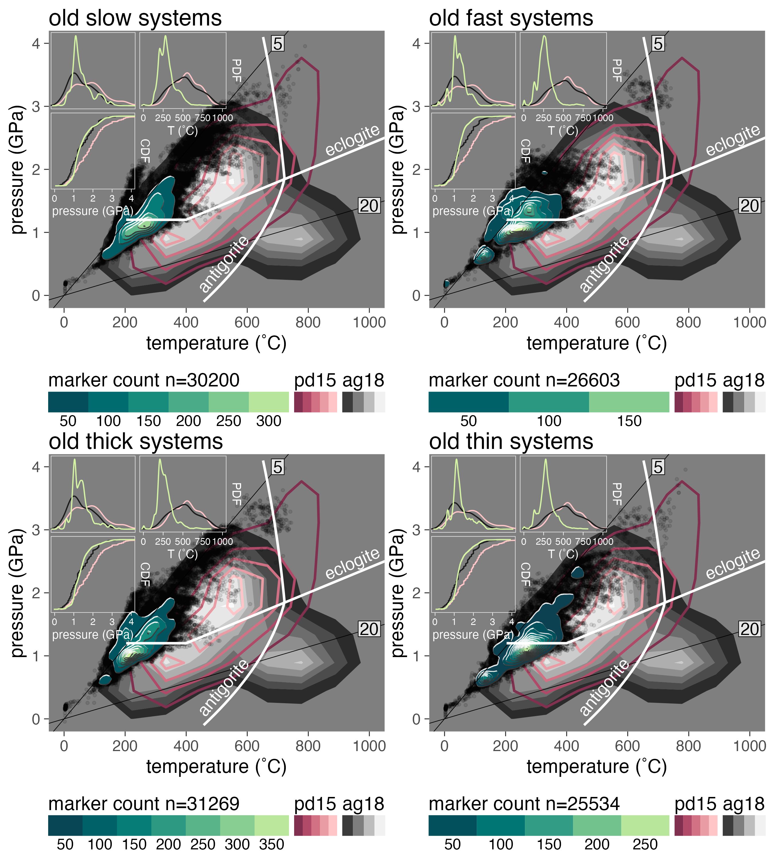
Figure 4.6: PT diagram showing the PT conditions of recovered markers (black point coulds) from numerical experiments with older oceanic plates (85-110 Ma) and the frequencies of recovered markers (green Tanaka contours) in comparison with the pd15 (solid red contours) and ag18 (filled gray contours) datasets, grouped by subduction zone setting (16 experiments per plot; boundary conditions summarized in Kerswell et al., 2021). Thin lines are thermal gradients labeled in ˚C/km. Reaction boundaries for eclogitization of oceanic crust and antigorite dehydration are from Ito & Kennedy (1971) and Schmidt & Poli (1998), respectively. Marker counts (Tanaka contours) are computed across a 100 \(\times\) 100 grid (0.04 GPa \(\times\) 10 ˚C). (insets) Probability distribution functions (top insets) and cumulative distribution functions (bottom inset) comparing P and T distributions between numerical experiments (green lines) and natural samples (pink lines: pd15, black lines: ag18).

4.3.2 Markers vs. Subduction Zone Settings

4.3.2.1 Oceanic Plate Age Effect

Thermal gradients of recovered markers respond strongly to changes in oceanic plate age (Figure 4.7, Table C.1). Both PT gradient modes are strongly inversely correlated with oceanic plate age, showing a mean increase from about 5.88 ± 0.16 ˚C/km (Grad mode1) and 6.99 ± 0.71 ˚C/km (Grad mode2) for older plates (≥ 85 Ma) to about 7.24 ± 0.05 ˚C/km (Grad mode1) and 8.81 ± 0.57 ˚C/km (Grad mode2) for younger plates (≤ 55 Ma). The dominant P mode (P mode1) moderately correlates with oceanic plate age, indicating a slightly higher possibility of recovering material from beyond the continental Moho for the oldest oceanic plates (≥ 85 Ma). Neither T modes, nor recovery rate correlate with oceanic plate age. Although oceanic plate age strongly affects the average PT gradients of recovered material, it does not strongly shift marker recovery up or down the subduction interface (e.g., compare average thermal gradients of markers between Figures 4.5 and 4.6).

4.3.2.2 Convergence Velocity Effect

P’s and T’s of recovered markers respond strongly to changes in convergence velocity (Figure 4.7, Table C.1). Both P modes are strongly inversely correlated with convergence velocity, showing a mean increase from 1.08 ± 0.04 GPa (P mode1) and 1.92 ± 0.44 GPa (P mode2) for fast moving plates (100 km/Ma) to about 1.38 ± 0.11 GPa (P mode1) and 2.63 ± 0.13 GPa (P mode2) for slow moving plates (40 km/Ma). However, the dominant P mode (P mode1) does not change significantly until convergence velocity drops below 66 km/Ma (Table C.1). Both T modes are strongly inversely correlated with convergence velocity, showing a mean increase from 250.2 ± 7.3 ˚C (T mode1) and 372.3 ± 74.2 ˚C (T mode2) for fast moving plates (100 km/Ma) to about 311.6 ± 1.6 ˚C (T mode1) and 546 ± 78 ˚C (T mode2) for slow moving plates (40 km/Ma). Neither PT gradient modes, nor recovery rate correlate with convergence velocity. In summary, decreasing convergence velocity shifts marker recovery to warmer and deeper conditions along the subduction interface without significantly changing the average thermal gradient of subducted material.

4.3.2.3 Upper-plate Thickness Effect

A strong positive association between upper-plate thickness and mechanical coupling depths was demonstrated for the same numerical experiments used to trace markers (Kerswell et al., 2021). P distributions of markers were thus expected to respond strongly to changes in upper-plate thickness. However, a surprisingly negligible effect was observed (Figure 4.7). For example, neither of the P modes, nor T mode2 or Grad mode2 (usually the most deeply subducted markers) correlate with upper-plate thickness. In contrast, the dominant PT gradient mode (Grad mode1) and T mode (T mode1) inversely correlate with upper-plate thickness. Recovery rate (ratio of recovered:subducted markers) is correlated with upper-plate thickness and not with any other boundary condition, indicating higher recovery rates are more likely underneath thick upper-plates. Recovery rates show a mean decrease from 10.66 ± 0.26 % for thicker plates (≥ 78 km-thick) to 8.08 ± 0.3 % for thinner upper-plates (≤ 62 km-thick). In summary, thin upper-plates are more likely to produce warmer thermal gradients, higher T’s, and lower recovery rates.

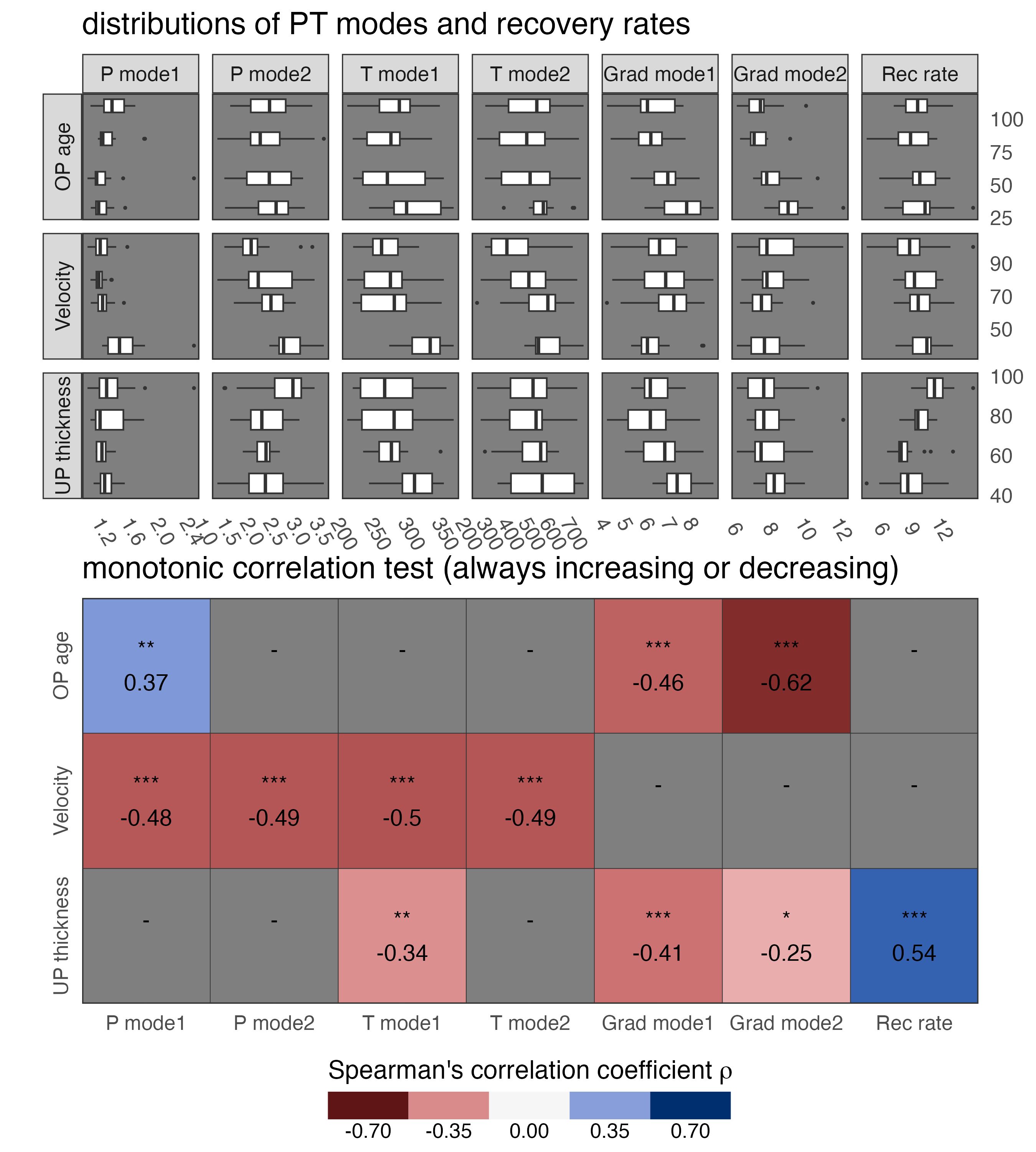
Figure 4.7: (top) Distributions of marker recovery modes and recovery rates for all numerical experiments (Table C.1). (bottom) Correlations among marker recovery modes and subduction zone settings. The dominant recovery mode (mode1) indicates the position of the tallest frequency peak with respect to P, T, or thermal gradient (i.e., conditions from which the greatest number of markers are recovered), while mode2 indicates the position of the warmest, deepest, or highest PT gradient frequency peak (i.e., conditions from which very few deeply subducted markers are recovered; typically \(\leq\) 1–10% the number of markers in mode1). Symbols indicate the Spearman’s rank correlation coefficient that measures the significance of monotonic correlations. *** \(\rho \leq\) 0.001 (99.9% confidence), ** \(\rho \leq\) 0.01 (99% confidence), * \(\rho \leq\) 0.05 (95% confidence), - \(\rho \geq\) 0.05 (< 95% confidence).

4.4 Discussion

4.4.1 Thermo-Kinematic Controls on Rock Recovery

While the combined distribution of markers recovered from all numerical experiments shows appreciable deviations from PT estimates compiled by Penniston-Dorland et al. (2015) and Agard et al. (2018), markers recovered from simulations with the youngest oceanic plates (32.6-55 Ma) and the slowest convergence velocities (40-66 km/Ma) begin to resemble the distribution of exhumed HP rocks with respect to thermal gradients and P distributions (compare Figure 4.4 with Figures 4.5 and 4.6). Slower subduction of younger plates increases marker thermal gradients and strongly shifts marker recovery down the subduction interface (strong correlations with Grad and P modes, Figure 4.7). For example, experiments with the slowest convergence velocities have P CDF’s that resemble ag18. It is important to note that old systems (with thin and thick upper-plates) also resemble ag18 with respect to their P CDF’s, while on the other hand, all experiments deviate strongly from pd15 with respect to their P CDF’s and show considerable thermal discrepancies with both pd15 and ag18 (especially lacking recovered markers above 525 ˚C), regardless of thermo-kinematic boundary conditions (Figure 4.5 and 4.6).

The correlations in Figure 4.7 suggest a shift towards warmer recovery conditions could be complemented by thin upper-plates—implying systems with thin upper-plates, slow convergence, and young oceanic plates should be the most consistent with the distribution of rock recovery implied by pd15 and ag18 (Figure 4.5). This correspondence might appear consistent with arguments that the rock record is composed primarily of rock bodies exhumed from “warm” subduction settings (i.e., geodynamic bias, Abers et al., 2017; van Keken et al., 2018). However, our numerical experiments also show that recovery rates do not correlate with oceanic plate age or convergence velocity, and that recovery rates are poorer for thinner upper-plates (Figure 4.7). Poor correlations among recovery rates and important subduction zone parameters (except for upper-plate thickness) suggest that rock recovery, in terms of volumes of recovered material, is not largely dependent on subduction zone setting. The many tens of thousands of markers recovered from a wide variety of numerical experiments summarized in Figure 4.7 counter the notion that greater volumes of rock are preferentially recovered from “warm” subduction zone settings. However, since our analysis focused on recovery, rather than exhumation, we cannot rule out the possibility of preferential exhumation from certain PT conditions that might be implicitly represented in ag18 and pd15.

Besides recovery rates of subducting markers, other dynamic characteristics appear to correlate with oceanic plate age and convergence velocity. For example, simulations with slow convergence velocities (e.g., models: cda, cde, cdi, cdm) tend to have higher subduction angles (see Appendix C.3) with thicker subduction interfaces that allow more markers to subduct to deeper, and thus warmer, conditions compared to other experiments (e.g., models: cdd, cdh, cdl, cdp) that form narrow interfaces with shallow choke points (e.g., see Appendix C.3). Observationally, the angle of subduction does not correlate significantly with oceanic plate age or convergence velocity, but rather inversely with the duration of subduction (Hu & Gurnis, 2020). Thus, the rock record might indicate preferential exhumation during the earlier stages of subduction when subduction angles were steeper (although not necessarily during subduction initiation), even for older oceanic plates. More generally, differences in plate flexibility, overall subduction geometry, and velocity of plate motions strongly affect PT distributions of rock recovery (Monie & Agard, 2009)—rather than strictly “warm” versus “cool” subduction settings per se. In other words, thermo-kinematic boundary conditions typically inferred to strictly regulate thermal effects (e.g., young-slow oceanic plates supporting warmer thermal gradients) may indeed be regulating more dynamic effects (e.g., young-slow oceanic plates flexibly rolling back to support deeper subduction of material along thicker interfaces) that are subsequently observed as thermal effects (average increase in marker PTs).

4.4.2 Comparison with other Numerical Experiments

Marker PT distributions and their correlations with thermo-kinematic boundary conditions presented above are determined directly from large samples of recovered material evolving dynamically in a deforming subduction interface (analogous to reconstructing thermal gradients from large random samples of exhumed HP rocks). In contrast, other studies investigating thermal responses to variable boundary conditions typically determine PT gradients statically along discrete surfaces representing megathrust faults (e.g., Abers et al., 2006; Currie et al., 2004; Davies, 1999a; Furukawa, 1993; Gao & Wang, 2014; McKenzie, 1969; Molnar & England, 1990; Peacock & Wang, 1999; Syracuse et al., 2010; van Keken et al., 2011, 2019; Wada & Wang, 2009) or dynamically by “finding” the subduction interface heuristically at each timestep (e.g., Arcay, 2017; Holt & Condit, 2021; Ruh et al., 2015). Other studies using similar geodynamic codes have traced many fewer markers (typically dozens vs. \(\sim\) 120,000; Faccenda et al., 2008; Gerya et al., 2002; Sizova et al., 2010; Yamato et al., 2007, 2008) from a narrower range of subduction zone settings, so they have less statistical rigor. This study stresses the importance of large sample sizes because individual marker PT paths can vary considerably within a single simulation. Important modes of recovery become apparent from high-frequency peaks only as more markers are traced. Furthermore, most other studies make no attempt to determine peak PT conditions related to detachment (but with some important exceptions, e.g., Roda et al., 2012, 2020), so marker PT paths are less analogous to PT paths determined by applying petrologic modeling.

4.4.3 Comparison with Geophysical Observations

The locations of important recovery modes determined from numerical experiments correspond closely with the depths of important mechanical transitions inferred from seismic imaging studies and surface heat flow observations. For example, the dominant recovery mode common among all numerical experiments at about 1 GPa (Table C.1 and Figure 4.4) is consistent with a layer of low seismic velocities and high \(V_p/V_s\) ratios observed at numerous subduction zones between 20-50 km depth (Bostock, 2013). While considerable unknowns persist about the nature of deformation in this region (Bostock, 2013; Tewksbury-Christle & Behr, 2021), the low-velocity zone, accompanied by low-frequency and slow-slip seismic events, is often interpreted as a transitional brittle-ductile shear zone that actively accommodates underplating of subducted material and/or formation of a tectonic mélange around the base of the continental Moho (Audet & Kim, 2016; Audet & Schaeffer, 2018; Bostock, 2013; Calvert et al., 2011, 2020; Delph et al., 2021).

Formation of low-velocity zones and their geophysical properties are generally attributed to high pore-fluid pressures caused by metamorphic reactions relating to the dehydration of oceanic crust (Hacker, 2008; Rondenay et al., 2008; van Keken et al., 2011). Surprisingly, despite our numerical implementation of a relatively simple model for dehydration of oceanic crust (Ito & Kennedy, 1971; Kerswell et al., 2021), and a relatively simple visco-plastic rheological model (Gerya & Yuen, 2003; Kerswell et al., 2021), the primary mode of marker recovery at 1.15 ± 0.46 GPa (2 \(\sigma\), Table C.1) coincides closely with the expected region for shallow underplating according to geophysical constraints (35 ± 15 km or 1.0 ± 0.4 GPa). The size of the markers dataset (n = 119,146 recovered markers) and prevalence of marker recovery from 1 GPa suggest that although dehydration may indeed trigger detachment of subducting rocks, other factors—notably the compositional and mechanical transition in the upper-plate across the Moho—also influence detachment at this depth.

The termination of the low-velocity zone at depths beyond the continental Moho marks another important mechanical transition. This second transition is often interpreted as the onset of mechanical plate coupling near 80 km (or 2.3 GPa, Agard et al., 2009, 2018; Furukawa, 1993; Monie & Agard, 2009; Plunder et al., 2015; Wada & Wang, 2009) and coincides well with the deeper recovery modes (P mode2) of markers at 2.2 ± 1.1 GPa (2 \(\sigma\), Table C.1). Although these deeper modes of marker recovery from near 2 GPa are noticeable in our numerical experiments and consistent with maximum recovery depths implied in pd15 and ag18, they represent a minor fraction of recovered markers—typically \(\leq\) 1–10% for individual numerical experiments. In other words, markers indicate maximum recovery depths that are consistent with the onset of plate coupling, but the relative frequency of material recovered from near 2 GPa in numerical experiments is inconsistent with the amount of material represented in pd15 and ag18 from the same conditions. Between the major mode of recovery at \(\sim\) 35–40 km and the few markers recovered from near \(\sim\) 80 km lies a gap in (or significant lack of) recovered markers that coincides with the highest sample frequencies of exhumed HP rocks compiled in pd15 and ag18 (Figure 4.4). This recovery gap is discussed in the following section.

4.4.4 The Marker Recovery Gap

Although recovered markers partially overlap with the range of PT estimates compiled in the pd15 and ag18 datasets, the differences between distributions of recovered markers and natural samples are numerous, including: (1) an obvious lack of markers recovered from ≥ 15 ˚C/km (0.001%) compared to pd15 and ag18 (37-48%, Figure 4.4), (2) recovery of markers from a single dominant mode near 1 GPa and 275 ˚C compared to more broadly distributed multimodal recovery across PT space for natural samples (Figure 4.4), (3) a general shift towards lower T’s and cooler thermal gradients for markers compared to natural samples, and (4) a remarkable gap in marker recovery near 2 GPa and 550 ˚C that coincides with the highest frequency of natural samples (Figure 4.4). In fact, across 64 numerical experiments with wide-ranging initial conditions less than 1% (0.65%) of markers are recovered from between 1.8-2.2 GPa and 475-625 ˚C. Why might this gap occur? Four possibilities are considered:

1. Simple rheological models preclude certain recovery mechanisms (poor implementation of subduction interface mechanics, i.e., modeling uncertainty, Section 4.4.4.1)
2. Peak metamorphic conditions are systematically misinterpreted (peak metamorphic conditions do not correspond to maxP or PT paths are not well constrained, i.e., petrologic uncertainties, Section 4.4.4.2, e.g., see Penniston-Dorland et al., 2015)
3. Rocks are frequently (re)sampled from the same peak metamorphic conditions and other rocks from different metamorphic grades are infrequently sampled (selective nonrandom sampling, i.e., scientific bias, Section 4.4.4.3, e.g., see Agard et al., 2018)
4. Rocks are recovered during short-lived events (e.g., subduction of seamounts, Agard et al., 2009) or by preferential exhumation mechanisms that are not implemented in our numerical experiments, rather than recovered during steady-state subduction within a serpentine-rich tectonic mélange that is characteristic of our numerical experiments (i.e., geodynamic uncertainties, Section 4.4.4.4)

4.4.4.1 Numerical Modeling Uncertainties

Simplifying assumptions in our numerical experiments influence thermal gradients and dynamics of rock recovery from the subducting oceanic plate. Substantially lower T’s and thermal gradients in numerical experiments compared to natural samples (Figure 4.4) might indicate imperfect implementation of heat generation and transfer (Kohn et al., 2018; Penniston-Dorland et al., 2015). In the numerical experiments, our rheological model and implementation of serpentine formation in the upper mantle creates a weak interface. A stronger rheology (e.g., quartz or a mixed melange zone, Beall et al., 2019; Ioannidi et al., 2021), or a stronger serpentine flow law (Burdette & Hirth, 2022), would yield greater heating and higher T’s from enhanced viscous dissipation (calculated as the product of deviatoric stress and strain rate in our experiments, Gerya, 2019) along the subduction interface (similar to increasing shear heating, e.g., Kohn et al., 2018). In principle, a stronger rheology might shift the overall PT distribution of markers to higher T’s and help fill in the marker recovery gap around 2 GPa and 550 ˚C, and/or possibly change flow to extract rocks more broadly along the subduction interface. Although the effects of different interface rheologies on thermal structure or rock recovery were not explicitly explored in this study, we note that numerical simulations with the smallest PT discrepancies between markers and natural samples (youngest oceanic plates and slowest convergence velocities, Figures 4.5 and 4.6) exhibit the same sizeable gap in marker recovery around 2 GPa and 550 ˚C. Thus, higher T’s alone would not seem to close the gap.

Stronger interface rheologies would also change the distribution of strain within the interface shear zone and likely induce interface migration due to stronger coupling mechanics (e.g., Agard et al., 2020). Recovery rates and the P (depth) distributions of recovered rocks are therefore expected to be affected by interface strength, in addition to temperature. However, the geodynamics of coupling and interface migration are more complex than thermal effects. For example, it is possible to analytically predict the temperature increase due to viscous dissipation by evaluating the stress and strain rate terms in empirical flow laws for various viscosities (material strengths). On the other hand, it is not possible to analytically predict changes to interface morphology, position, or strain distribution as a function of rheological parameters. Numerical experiments are necessary to evaluate such complex geodynamic phenomena, so we propose a more systematic study of the effects of various interface rheologies on rock recovery as a topic for future research.

4.4.4.2 Petrologic Uncertainties

Interpreting peak metamorphic conditions of complex polymetamorphic rocks is challenging with many sources of uncertainties. However, a global shift in PT estimates of natural samples towards warmer conditions compared to recovered markers would imply that decades of field observations, conventional thermobarometry (e.g., Spear & Selverstone, 1983), phase equilibria modeling (e.g., Connolly, 2005), trace element thermometry (e.g., Ferry & Watson, 2007; Kohn, 2020), and Raman Spectroscopy of Carbonaceous Material thermometry (Beyssac et al., 2002) from many independent localities worldwide (e.g., Agard et al., 2009, 2018; Angiboust et al., 2009, 2012a, 2016; Avigad & Garfunkel, 1991; Monie & Agard, 2009; Plunder et al., 2013, 2015) have systematically misinterpreted the prograde and retrograde histories of exhumed HP rocks. The consistency of independent analytical techniques suggests systematic bias is unlikely and estimated uncertainties are generally too small for this argument to be viable (Penniston-Dorland et al., 2015).

4.4.4.3 Selective Sampling and Scientific Bias

At least two factors might lead to scientific bias. First, the application of conventional thermobarometry is easier for certain rock types and mineral assemblages (e.g., eclogite-facies metabasites and metapelitic schists) than for others (e.g., quartzites, metagraywackes). Second, certain subduction complexes expose more rocks than others. These factors lead to sampling bias, both in the rocks that are selected for analysis and which subduction complexes contribute most to compilations. For example, a PT condition of \(\sim\) 2 GPa and 550 ˚C typically yields assemblages that are both recognizable in the field (eclogites, sensu stricto, and kyanite- or chloritoid-schists) and amenable to thermobarometric calculations and petrologic modeling. This fact may lead to oversampling of the rocks that yield these PT conditions and the subduction zones that expose these rocks. In Penniston-Dorland et al. (2015), the western and central European Alps, which contain many rocks that equilibrated near this PT condition, represented \(\sim\) 90 samples across < 1000 km (\(\sim\) 1 sample per 10 km), whereas the Himalaya and Andes, which contained more diverse PT conditions, represented only \(\sim\) 1 sample per 300-400 km. Some subduction zones are not represented at all in these datasets (e.g., central and western Aleutians, Kamchatka, Izu-Bonin-Marianas, Philippines, Indonesia, Tonga-Kermadec, etc.), either because metamorphic rocks are not exposed (that we know of) or rock types are not amenable to petrologic investigation. Correcting for this type of bias is challenging because it would require large random samples of exhumed HP rocks from localities worldwide and development of new techniques for quantifying PT conditions in diverse rock types.

4.4.4.4 Short-lived Events and Geodynamic Uncertainties

Detachment of rocks from the subducting slab might not occur randomly, but rather in response to specific events, such as subduction of asperities or seamounts (e.g., Agard et al., 2009) or abrupt fluid events. Yet no numerical models have attempted to model these events. In the case of seamounts, high surface roughness correlates with higher coefficients of friction (Gao & Wang, 2014). Higher friction increases heating and T’s, driving subduction interface thermal gradients into the field of PT conditions defined by the pd15 and ag18 datasets (Kohn et al., 2018). If asperities become mechanically unstable at depths of \(\sim\) 50-70 km, preferential detachment would create an “overabundance” of recorded PT conditions at moderate T (\(\sim\) 550 ˚C) at \(\sim\) 2 GPa, as observed.

Alternatively, although fluid release is modeled in our numerical experiments as continuous, it may occur sporadically in nature (Audet et al., 2009; Faccenda, 2014). Two dehydration reactions along the subduction interface that are particularly relevant, but not explicitly modeled in the numerical experiments are: the transformation of lawsonite to epidote, and the transformation of chlorite (plus quartz) to garnet (e.g., Angiboust & Agard, 2010; Baxter & Caddick, 2013; Vitale Brovarone & Agard, 2013). Although dehydration of lawsonite is nearly discontinuous in PT space, few rocks show clear evidence for lawsonite immediately prior to peak metamorphism (although such evidence can be subtle). In the context of equilibrium thermodynamics, chlorite dehydration should occur continuously below depths of \(\sim\) 35 km (Baxter & Caddick, 2013; Schmidt & Poli, 1998, 2013), consistent with assumptions of many numerical geodynamic models. However, some research suggests substantial overstepping of this reaction, resulting in the abrupt formation of abundant garnet and release of water (Castro & Spear, 2017). Direct geochronology of garnet growth rates in subduction complexes also suggests rapid growth and water release (Dragovic et al., 2015). Because fluids are thought to help trigger brittle failure (earthquakes) that could detach rocks from the subducting slab surface, abrupt water release at a depth of \(\sim\) 50-70 km might again result in an “overabundance” of recorded PT conditions at P’s of \(\sim\) 2 GPa. However, this explanation for abundant recovery of material from near 2 GPa would not directly explain higher T’s, and would require relatively consistent degrees of overstepping in rocks of similar bulk composition, despite differences in subduction parameters (such as subduction rate) that must control rates of P- and T-increase. Similar to the proposed investigations regarding various interface rheologies (Section 4.4.4.1), a more systematic study of the effects of various dehydration reactions on rock recovery is possible with numerical geodynamic models and should be a topic for future research.

4.5 Conclusions

This study traces PT paths of more than one million markers from 64 subduction simulations representing a large range of presently active subduction zones worldwide. Marker recovery is identified by implementing a “soft” clustering algorithm, and PT distributions of recovered markers are compared among models and with the rock record. Such a large dataset presents a statistically-robust portrait of important recovery modes (conditions under which most markers are detached) along the subduction interface. The three most important findings are as follows:

1. Numerical simulations with relatively simple (de)hydration models and visco-plastic interface rheologies simulate important recovery mechanisms near the base of the continental Moho around 1 GPa and 275 ˚C (underplating and/or formation of tectonic mélanges) and near the depth of mechanical plate coupling around 2.3–2.5 GPa and 525 ˚C. The pd15 and ag18 datasets also indicate preferential recovery near \(\sim\) 1 GPa, although the frequency of samples is much lower than model predictions.
2. Subduction systems with young oceanic plates, slow convergence velocities, and thin upper-plate lithospheres are most consistent with the rock record, but it is unclear to what extent kinematic effects (young flexible oceanic plates with high subduction angles accommodating deeper subduction of material) rather than thermal effects (young oceanic plates supporting higher thermal gradients) drive changes in marker PT distributions. Comparing PT distributions of recovered markers from young-slow-thin numerical experiments with the rock record is not straightforward, however, because numerical experiments also indicate that recovery rates do not correlate with oceanic plate age or convergence velocity, and fewer markers are recovered from subduction systems with thin upper-plates.
3. While maximum marker recovery depths near 2.3–2.5 GPa in many numerical experiments is consistent with the onset of plate coupling and sudden decrease in sample frequency above 2.3–2.5 GPa in the rock record, very few markers are recovered from 1 GPa. A gap in (or significant lack of) marker recovery near 2 GPa and 550 ˚C contrasts with the high frequencies of natural samples at this approximate PT condition. Explanations for this “overabundance” of natural samples might include selective sampling of rocks amenable to petrologic investigation (sampling bias), reaction overstepping (abrupt release of water triggering detachment of rock near 2 GPa and 550 ˚C), or processes such as subduction of seamounts or exhumation mechanisms that are not included in numerical simulations. Future work targeting natural samples from a larger range of peak PT conditions and analyzing marker recovery from numerical geodynamic models that include new implementations of metamorphic (de)hydration reactions and interface rheologies might help resolve this discrepancy.

5 Conclusion

This work uses three computational approaches—simulation, interpolation, and applied statistics (machine learning)—to address the following questions. How does plate interface mechanics change across a range of subduction zones and how can it be quantified with currently available petrologic and geophysical datasets?

Plate coupling observed in numerical simulations from Chapter 2 demonstrate steady-state mechanical behavior regulated self-consistently by feedbacks involving heat transfer and metamorphic dehydration of ultramafic sheet silicates in the upper-plate mantle. Coupling depth is only weakly correlated with \(\Phi\) but strongly correlated with upper-plate lithospheric thickness. Thus uniform coupling depths are expected if subduction zones have uniformly thick upper-plates, which is indeed the case when considering averaged backarc surface heat flow for 13 presently active subduction zones (Currie et al., 2004; Currie & Hyndman, 2006; Hyndman et al., 2005; Wada & Wang, 2009).

However, surface heat flow interpolations in Chapter 3 show a Kaleidoscope of upper-plate surface heat flow patterns—some implying continuous thermal structure, others implying discontinuous thermal structure—for 13 presently active subduction zones. While Kriging methods yield some spurious results for segments with low observational densities, both Similarity and Kriging methods indicate comparable accuracy rates on average. Thus both methods are ostensibly suitable for subduction zone research if carefully applied. Further, differences between Similarity and Kriging predictions highlight anomalies and point towards effective sampling strategies for future surveys.

Chapter 4 takes a different approach by considering what PT distributions of exhumed HP metamorphic rocks imply about mechanical variability among subduction zones with respect to detachment (recovery) of subducted materials. A large (119,146) dataset of recovered markers shows marker PT distributions and recovery rates correlate with certain thermo-kinematic boundary conditions (oceanic plate age, convergence velocity, and upper-plate thickness) and indicate a range of plausible conditions for reproducing the rock record. A sizeable gap in marker recovery around 2 GPa and 550 ˚C, coinciding with the highest density of natural samples, implies biases (including imperfect implementation of recovery mechanisms in numerical experiments, sampling biases, and reaction overstepping) may be strongly affecting the rock record and/or numerical geodynamic models.

Future work may focus on refining and improving numerical geodynamic codes (to better implement heat generation/transfer and recovery mechanisms), surface heat flow datasets (to improve interpolation accuracies), and petrologic datasets (to enable sampling and modelling of more diverse rock types) by exploring and addressing the potential biases identified in the above studies.

References

Abers, G., Keken, P. van, Kneller, E., Ferris, A., & Stachnik, J. (2006). The thermal structure of subduction zones constrained by seismic imaging: Implications for slab dehydration and wedge flow. Earth and Planetary Science Letters, 241(3-4), 387–397.

Abers, G., van Keken, P., & Hacker, B. (2017). The cold and relatively dry nature of mantle forearcs in subduction zones. Nature Geoscience, 10(5), 333–337.

Abers, G., Keken, P. van, & Wilson, C. (2020). Deep decoupling in subduction zones: Observations and temperature limits. Geosphere, 16(6), 1408–1424.

Agard, P. (2021). Subduction of oceanic lithosphere in the alps: Selective and archetypal from (slow-spreading) oceans. Earth-Science Reviews, 214, 103517.

Agard, P., Yamato, P., Jolivet, L., & Burov, E. (2009). Exhumation of oceanic blueschists and eclogites in subduction zones: Timing and mechanisms. Earth-Science Reviews, 92(1-2), 53–79.

Agard, P., Yamato, P., Soret, M., Prigent, C., Guillot, S., Plunder, A., et al. (2016). Plate interface rheological switches during subduction infancy: Control on slab penetration and metamorphic sole formation. Earth and Planetary Science Letters, 451, 208–220.

Agard, P., Plunder, A., Angiboust, S., Bonnet, G., & Ruh, J. (2018). The subduction plate interface: Rock record and mechanical coupling (from long to short time scales). Lithos, 320-321, 537–566.

Agard, P., Prigent, C., Soret, M., Dubacq, B., Guillot, S., & Deldicque, D. (2020). Slabitization: Mechanisms controlling subduction development and viscous coupling. Earth-Science Reviews, 208, 103259.

Agrusta, R., Arcay, D., Tommasi, A., Davaille, A., Ribe, N., & Gerya, T. (2013). Small-scale convection in a plume-fed low-viscosity layer beneath a moving plate. Geophysical Journal International, 194(2), 591–610.

Angiboust, S., & Agard, P. (2010). Initial water budget: The key to detaching large volumes of eclogitized oceanic crust along the subduction channel? Lithos, 120(3-4), 453–474.

Angiboust, S., Agard, P., Jolivet, L., & Beyssac, O. (2009). The zermatt-saas ophiolite: The largest (60-km wide) and deepest (c. 70–80 km) continuous slice of oceanic lithosphere detached from a subduction zone? Terra Nova, 21(3), 171–180.

Angiboust, S., Agard, P., Raimbourg, H., Yamato, P., & Huet, B. (2011). Subduction interface processes recorded by eclogite-facies shear zones (monviso, w. alps). Lithos, 127(1-2), 222–238.

Angiboust, S., Langdon, R., Agard, P., Waters, D., & Chopin, C. (2012a). Eclogitization of the monviso ophiolite (w. Alps) and implications on subduction dynamics. Journal of Metamorphic Geology, 30(1), 37–61.

Angiboust, S., Wolf, S., Burov, E., Agard, P., & Yamato, P. (2012b). Effect of fluid circulation on subduction interface tectonic processes: Insights from thermo-mechanical numerical modelling. Earth and Planetary Science Letters, 357, 238–248.

Angiboust, S., Pettke, T., De Hoog, J., Caron, B., & Oncken, O. (2014a). Channelized fluid flow and eclogite-facies metasomatism along the subduction shear zone. Journal of Petrology, 55(5), 883–916.

Angiboust, S., Glodny, J., Oncken, O., & Chopin, C. (2014b). In search of transient subduction interfaces in the dent blanche–sesia tectonic system (w. alps). Lithos, 205, 298–321.

Angiboust, S., Kirsch, J., Oncken, O., Glodny, J., Monié, P., & Rybacki, E. (2015). Probing the transition between seismically coupled and decoupled segments along an ancient subduction interface. Geochemistry, Geophysics, Geosystems, 16(6), 1905–1922.

Angiboust, S., Agard, P., Glodny, J., Omrani, J., & Oncken, O. (2016). Zagros blueschists: Episodic underplating and long-lived cooling of a subduction zone. Earth and Planetary Science Letters, 443, 48–58.

Arcay, D. (2017). Modelling the interplate domain in thermo-mechanical simulations of subduction: Critical effects of resolution and rheology, and consequences on wet mantle melting. Physics of the Earth and Planetary Interiors, 269, 112–132.

Arcay, D., Doin, M., Tric, E., Bousquet, R., & de Capitani, C. (2006). Overriding plate thinning in subduction zones: Localized convection induced by slab dehydration. Geochemistry, Geophysics, Geosystems, 7(2).

Audet, P., & Kim, Y. (2016). Teleseismic constraints on the geological environment of deep episodic slow earthquakes in subduction zone forearcs: A review. Tectonophysics, 670, 1–15.

Audet, P., & Schaeffer, A. (2018). Fluid pressure and shear zone development over the locked to slow slip region in cascadia. Science Advances, 4(3), eaar2982.

Audet, P., Bostock, M., Christensen, N., & Peacock, S. (2009). Seismic evidence for overpressured subducted oceanic crust and megathrust fault sealing. Nature, 457(7225), 76–78.

Avigad, D., & Garfunkel, Z. (1991). Uplift and exhumation of high-pressure metamorphic terrains: The example of the cycladic blueschist belt (aegean sea). Tectonophysics, 188(3-4), 357–372.

Banfield, J., & Raftery, A. (1993). Model-based gaussian and non-gaussian clustering. Biometrics, 803–821.

Bárdossy, A. (1997). Introduction to geostatistics. Institute of Hydraulic Engineering, University of Stuttgart.

Barlow, H. (1989). Unsupervised learning. Neural Computation, 1(3), 295–311.

Batchelor, G. (1953). The theory of homogeneous turbulence. Cambridge university press.

Baxter, E., & Caddick, M. (2013). Garnet growth as a proxy for progressive subduction zone dehydration. Geology, 41(6), 643–646.

Beall, A., Fagereng, Å., & Ellis, S. (2019). Strength of strained two-phase mixtures: Application to rapid creep and stress amplification in subduction zone mélange. Geophysical Research Letters, 46(1), 169–178.

Bebout, G. (2007). Metamorphic chemical geodynamics of subduction zones. Earth and Planetary Science Letters, 260(3-4), 373–393.

Bebout, G., & Barton, M. (2002). Tectonic and metasomatic mixing in a high-t, subduction-zone mélange—insights into the geochemical evolution of the slab–mantle interface. Chemical Geology, 187(1-2), 79–106.

Beyssac, O., Goffé, B., Chopin, C., & Rouzaud, J. (2002). Raman spectra of carbonaceous material in metasediments: A new geothermometer. Journal of Metamorphic Geology, 20(9), 859–871.

Bonnet, G., Agard, P., Angiboust, S., Monié, P., Jentzer, M., Omrani, J., et al. (2018). Tectonic slicing and mixing processes along the subduction interface: The sistan example (eastern iran). Lithos, 310, 269–287.

Bostock, M. (2013). The moho in subduction zones. Tectonophysics, 609, 547–557.

Boussinesq, J. (1897). Théorie de l’écoulement tourbillonnant et tumultueux des liquides dans les lits rectilignes a grande section (Vol. 1). Gauthier-Villars.

Bowen, N., & Tuttle, O. (1949). The system MgO—SiO2—H2O. Geological Society of America Bulletin, 60(3), 439–460.

Burdette, E., & Hirth, G. (2022). Creep rheology of antigorite: Experiments at subduction zone conditions. Journal of Geophysical Research: Solid Earth, 127(7), e2022JB024260.

Burg, J., & Gerya, T. (2005). The role of viscous heating in barrovian metamorphism of collisional orogens: Thermomechanical models and application to the lepontine dome in the central alps. Journal of Metamorphic Geology, 23(2), 75–95.

Burov, E., François, T., Agard, P., Le Pourhiet, L., Meyer, B., Tirel, C., et al. (2014). Rheological and geodynamic controls on the mechanisms of subduction and HP/UHP exhumation of crustal rocks during continental collision: Insights from numerical models. Tectonophysics, 631, 212–250.

Calvert, A., Preston, L., & Farahbod, A. (2011). Sedimentary underplating at the cascadia mantle-wedge corner revealed by seismic imaging. Nature Geoscience, 4(8), 545–548.

Calvert, A., Bostock, M., Savard, G., & Unsworth, M. (2020). Cascadia low frequency earthquakes at the base of an overpressured subduction shear zone. Nature Communications, 11(1), 1–10.

Carlson, R., & Miller, D. (2003). Mantle wedge water contents estimated from seismic velocities in partially serpentinized peridotites. Geophysical Research Letters, 30(5).

Castro, A., & Spear, F. (2017). Reaction overstepping and re-evaluation of peak p–t conditions of the blueschist unit sifnos, greece: Implications for the cyclades subduction zone. International Geology Review, 59(5-6), 548–562.

Celeux, G., & Govaert, G. (1995). Gaussian parsimonious clustering models. Pattern Recognition, 28(5), 781–793.

Chapman, D., & Pollack, H. (1975). Global heat flow: A new look. Earth and Planetary Science Letters, 28(1), 23–32.

Cisneros, M., Behr, W., Platt, J., & Anczkiewicz, R. (2022). Quartz-in-garnet barometry constraints on formation pressures of eclogites from the franciscan complex, california. Contributions to Mineralogy and Petrology, 177(1), 12.

Čížková, H., & Bina, C. (2013). Effects of mantle and subduction-interface rheologies on slab stagnation and trench rollback. Earth and Planetary Science Letters, 379, 95–103.

Cleveland, W., & Devlin, S. (1988). Locally weighted regression: An approach to regression analysis by local fitting. Journal of the American Statistical Association, 83(403), 596–610.

Cloos, M., & Shreve, R. (1988). Subduction-channel model of prism accretion, melange formation, sediment subduction, and subduction erosion at convergent plate margins: 1. Background and description. Pure and Applied Geophysics, 128(3), 455–500.

Connolly, J. (2005). Computation of phase equilibria by linear programming: A tool for geodynamic modeling and its application to subduction zone decarbonation. Earth and Planetary Science Letters, 236(1-2), 524–541.

Cressie, N. (2015). Statistics for spatial data. John Wiley & Sons.

Currie, C., & Hyndman, R. (2006). The thermal structure of subduction zone back arcs. Journal of Geophysical Research: Solid Earth, 111(B8), 1–22.

Currie, C., Wang, K., Hyndman, R., & He, J. (2004). The thermal effects of steady-state slab-driven mantle flow above a subducting plate: The cascadia subduction zone and backarc. Earth and Planetary Science Letters, 223(1-2), 35–48.

Davies, J. (1999a). Simple analytic model for subduction zone thermal structure. Geophysical Journal International, 139(3), 823–828.

Davies, J. (1999b). The role of hydraulic fractures and intermediate depth earthquakes in generating suduction zone magmatism. Nature, 417(March), 142–145.

Davies, J. (2013). Global map of solid earth surface heat flow. Geochemistry, Geophysics, Geosystems, 14(10), 4608–4622.

Davis, E., Hyndman, R., & Villinger, H. (1990). Rates of fluid expulsion across the northern cascadia accretionary prism: Constraints from new heat row and multichannel seismic reflection data. Journal of Geophysical Research: Solid Earth, 95(B6), 8869–8889.

Delph, J., Thomas, A., & Levander, A. (2021). Subcretionary tectonics: Linking variability in the expression of subduction along the cascadia forearc. Earth and Planetary Science Letters, 556, 116724.

Dempster, A., Laird, N., & Rubin, D. (1977). Maximum likelihood from incomplete data via the EM algorithm. Journal of the Royal Statistical Society: Series B (Methodological), 39(1), 1–22.

Dragovic, B., Baxter, E., & Caddick, M. (2015). Pulsed dehydration and garnet growth during subduction revealed by zoned garnet geochronology and thermodynamic modeling, sifnos, greece. Earth and Planetary Science Letters, 413, 111–122.

England, P., & Katz, R. (2010). Melting above the anhydrous solidus controls the location of volcanic arcs. Nature, 467(7316), 700–703.

England, P., Engdahl, R., & Thatcher, W. (2004). Systematic variation in the depths of slabs beneath arc volcanoes. Geophysical Journal International, 156(2), 377–408.

Faccenda, M. (2014). Water in the slab: A trilogy. Tectonophysics, 614, 1–30.

Faccenda, M., Gerya, T., & Chakraborty, S. (2008). Styles of post-subduction collisional orogeny: Influence of convergence velocity, crustal rheology and radiogenic heat production. Lithos, 103(1-2), 257–287.

Faccenda, M., Gerya, T., & Burlini, L. (2009). Deep slab hydration induced by bending-related variations in tectonic pressure. Nature Geoscience, 2(11), 790–793.

Ferris, A., Abers, G., Christensen, D., & Veenstra, E. (2003). High resolution image of the subducted pacific (?) plate beneath central alaska, 50–150 km depth. Earth and Planetary Science Letters, 214(3-4), 575–588.

Ferry, J., & Watson, E. (2007). New thermodynamic models and revised calibrations for the ti-in-zircon and zr-in-rutile thermometers. Contributions to Mineralogy and Petrology, 154(4), 429–437.

Festa, A., Pini, G., Ogata, K., & Dilek, Y. (2019). Diagnostic features and field-criteria in recognition of tectonic, sedimentary and diapiric mélanges in orogenic belts and exhumed subduction-accretion complexes. Gondwana Research, 74, 7–30.

Figueiredo, M., & Jain, A. (2002). Unsupervised learning of finite mixture models. IEEE Transactions on Pattern Analysis and Machine Intelligence, 24(3), 381–396.

Fisher, A., & Becker, K. (2000). Channelized fluid flow in oceanic crust reconciles heat-flow and permeability data. Nature, 403(6765), 71–74.

Fisher, D., Hooker, J., Smye, A., & Chen, T. (2021). Insights from the geological record of deformation along the subduction interface at depths of seismogenesis. Geosphere, 17(6), 1686–1703.

Fourier, J. (1827). Mémoire sur les températures du globe terrestre et des espaces planétaires. Mémoires de l’Académie Royale Des Sciences de l’Institut de France, 7, 570–604.

Fraley, C., & Raftery, A. (2002). Model-based clustering, discriminant analysis, and density estimation. Journal of the American Statistical Association, 97(458), 611–631.

Furlong, K., & Chapman, D. (2013). Heat flow, heat generation, and the thermal state of the lithosphere. Annual Review of Earth and Planetary Sciences, 41(1), 385–410.

Furukawa, Y. (1993). Depth of the decoupling plate interface and thermal structure under arcs. Journal of Geophysical Research: Solid Earth, 98(B11), 20005–20013.

Gao, X., & Wang, K. (2014). Strength of stick-slip and creeping subduction megathrusts from heat flow observations. Science, 345(6200), 1038–1041.

Gao, X., & Wang, K. (2017). Rheological separation of the megathrust seismogenic zone and episodic tremor and slip. Nature, 543(7645), 416–419.

Gerya, T. (2014). Precambrian geodynamics: Concepts and models. Gondwana Research, 25(2), 442–463.

Gerya, T. (2019). Introduction to numerical geodynamic modelling. Cambridge University Press.

Gerya, T., & Meilick, F. (2011). Geodynamic regimes of subduction under an active margin: Effects of rheological weakening by fluids and melts. Journal of Metamorphic Geology, 29(1), 7–31.

Gerya, T., & Stöckhert, B. (2006). Two-dimensional numerical modeling of tectonic and metamorphic histories at active continental margins. International Journal of Earth Sciences, 95(2), 250–274.

Gerya, T., & Yuen, D. (2003). Characteristics-based marker-in-cell method with conservative finite-differences schemes for modeling geological flows with strongly variable transport properties. Physics of the Earth and Planetary Interiors, 140(4), 293–318.

Gerya, T., Stöckhert, B., & Perchuk, A. (2002). Exhumation of high-pressure metamorphic rocks in a subduction channel: A numerical simulation. Tectonics, 21(6), 6–1.

Gerya, T., Connolly, J., & Yuen, D. (2008). Why is terrestrial subduction one-sided? Geology, 36(1), 43–46.

Gilio, M., Scambelluri, M., Agostini, S., Godard, M., Pettke, T., Agard, P., et al. (2020). Fingerprinting and relocating tectonic slices along the plate interface: Evidence from the lago superiore unit at monviso (western alps). Lithos, 352, 105308.

Gonzalez, C., Gorczyk, W., & Gerya, T. (2016). Decarbonation of subducting slabs: Insight from petrological–thermomechanical modeling. Gondwana Research, 36, 314–332.

Goodchild, M. (2004). The validity and usefulness of laws in geographic information science and geography. Annals of the Association of American Geographers, 94(2), 300–303.

Gorczyk, W., Willner, A., Gerya, T., Connolly, J., & Burg, J. (2007). Physical controls of magmatic productivity at pacific-type convergent margins: Numerical modelling. Physics of the Earth and Planetary Interiors, 163(1-4), 209–232.

Goutorbe, B., Poort, J., Lucazeau, F., & Raillard, S. (2011). Global heat flow trends resolved from multiple geological and geophysical proxies. Geophysical Journal International, 187(3), 1405–1419.

Gräler, B., Pebesma, E., & Heuvelink, G. (2016). Spatio-temporal interpolation using gstat. The R Journal, 8, 204–218. Retrieved from https://journal.r-project.org/archive/2016/RJ-2016-014/index.html

Groppo, C., Rolfo, F., Sachan, H., & Rai, S. (2016). Petrology of blueschist from the western himalaya (ladakh, NW india): Exploring the complex behavior of a lawsonite-bearing system in a paleo-accretionary setting. Lithos, 252, 41–56.

Grove, T., Till, C., & Krawczynski, M. (2012). The role of \(H_2O\) in subduction zone magmatism. Annual Review of Earth and Planetary Sciences, 40(1), 413–439.

Hacker, B. (1996). Eclogite formation and the rheology, buoyancy, seismicity, and h~ 2O content of oceanic crust. GEOPHYSICAL MONOGRAPH-AMERICAN GEOPHYSICAL UNION, 96, 337–346.

Hacker, B. (2008). H2O subduction beyond arcs. Geochemistry, Geophysics, Geosystems, 9(3).

Hacker, B., Abers, G., & Peacock, S. (2003). Subduction factory 1. Theoretical mineralogy, densities, seismic wave speeds, and \(H_2O\) contents. Journal of Geophysical Research: Solid Earth, 108(B1).

Harlow, F. (1962). The particle-in-cell method for numerical solution of problems in fluid dynamics. Los Alamos Scientific Lab., N. Mex.

Harlow, F. (1964). The particle-in-cell computing method for fluid dynamics. Methods Comput. Phys., 3, 319–343.

Harlow, F., & Welch, J. (1965). Numerical calculation of time-dependent viscous incompressible flow of fluid with free surface. The Physics of Fluids, 8(12), 2182–2189.

Harvey, K., Walker, S., Starr, P., Penniston-Dorland, S., Kohn, M., & Baxter, E. (2021). A mélange of subduction ages: Constraints on the timescale of shear zone development and underplating at the subduction interface, catalina schist (CA, USA). Geochemistry, Geophysics, Geosystems, 22(9), e2021GC009790.

Hasterok, D. (2013). A heat flow based cooling model for tectonic plates. Earth and Planetary Science Letters, 361, 34–43.

Hasterok, D., & Chapman, D. (2008). Global heat flow: A new database and a new approach. In AGU fall meeting abstracts (Vol. 2008, pp. T21c–1985).

Hasterok, D., Chapman, D., & Davis, E. (2011). Oceanic heat flow: Implications for global heat loss. Earth and Planetary Science Letters, 311(3-4), 386–395.

Hilairet, N., Reynard, B., Wang, Y., Daniel, I., Merkel, S., Nishiyama, N., & Petitgirard, S. (2007). High-pressure creep of serpentine, interseismic deformation, and initiation of subduction. Science, 318(5858), 1910–1913.

Hirauchi, K., Katayama, I., Uehara, S., Miyahara, M., & Takai, Y. (2010). Inhibition of subduction thrust earthquakes by low-temperature plastic flow in serpentine. Earth and Planetary Science Letters, 295(3-4), 349–357.

Holt, A., & Condit, C. (2021). Slab temperature evolution over the lifetime of a subduction zone. Geochemistry, Geophysics, Geosystems, e2020GC009476.

Hsü, K. (1968). Principles of mélanges and their bearing on the franciscan-knoxville paradox. Geological Society of America Bulletin, 79(8), 1063–1074.

Hu, J., & Gurnis, M. (2020). Subduction duration and slab dip. Geochemistry, Geophysics, Geosystems, 21(4), e2019GC008862.

Hutnak, M., Fisher, A., Harris, R., Stein, C., Wang, K., Spinelli, G., et al. (2008). Large heat and fluid fluxes driven through mid-plate outcrops on ocean crust. Nature Geoscience, 1(9), 611–614.

Hyndman, R., & Peacock, S. (2003). Serpentinization of the forearc mantle. Earth and Planetary Science Letters, 212(3-4), 417–432.

Hyndman, R., & Wang, K. (1993). Thermal constraints on the zone of major thrust earthquake failure: The cascadia subduction zone. Journal of Geophysical Research: Solid Earth, 98(B2), 2039–2060.

Hyndman, R., Currie, C., & Mazzotti, S. (2005). Subduction zone backarcs, mobile belts, and orogenic heat. GSA Today, 15(2), 4–10.

Ioannidi, P., Angiboust, S., Oncken, O., Agard, P., Glodny, J., & Sudo, M. (2020). Deformation along the roof of a fossil subduction interface in the transition zone below seismogenic coupling: The austroalpine case and new insights from the malenco massif (central alps). Geosphere, 16(2), 510–532.

Ioannidi, P., Le Pourhiet, L., Agard, P., Angiboust, S., & Oncken, O. (2021). Effective rheology of a two-phase subduction shear zone: Insights from numerical simple shear experiments and implications for subduction zone interfaces. Earth and Planetary Science Letters, 566, 116913.

Ito, K., & Kennedy, G. (1971). An experimental study of the basalt-garnet granulite-eclogite transition. The Structure and Physical Properties of the Earth’s Crust, 14, 303–314.

Jennings, S., Hasterok, D., & Lucazeau, F. (2021). ThermoGlobe: Extending the global heat flow database. Journal TBD.

Jull, M., & Kelemen, P. (2001). On the conditions for lower crustal convective instability. Journal of Geophysical Research: Solid Earth, 106(b4), 6423–6446.

Karato, S., & Wu, P. (1993). Rheology of the upper mantle: A synthesis. Science, 260(5109), 771–778.

Kelvin, W. (1863). On the secular cooling of the earth. Transactions of the Royal Society of Edinburgh, 23, 157–170.

Kerswell, B., Kohn, M., & Gerya, T. (2021). Backarc lithospheric thickness and serpentine stability control slab-mantle coupling depths in subduction zones. Geochemistry, Geophysics, Geosystems, 22(6), e2020GC009304.

Kirby, S., Durham, W., & Stern, L. (1991). Mantle phase changes and deep-earthquake faulting in subducting lithosphere. Science, 252(5003), 216–225.

Kitamura, Y., & Kimura, G. (2012). Dynamic role of tectonic mélange during interseismic process of plate boundary mega earthquakes. Tectonophysics, 568, 39–52.

Kohn, M. (2020). A refined zirconium-in-rutile thermometer. American Mineralogist: Journal of Earth and Planetary Materials, 105(6), 963–971.

Kohn, M., & Spear, F. (1991). Error propagation for barometers: 2. Application to rocks. American Mineralogist, 76(1-2), 138–147.

Kohn, M., Castro, A., Kerswell, B., Ranero, C. R., & Spear, F. (2018). Shear heating reconciles thermal models with the metamorphic rock record of subduction. Proceedings of the National Academy of Sciences, 115(46), 11706–11711.

Korgen, B., Bodvarsson, G., & Mesecar, R. (1971). Heat flow through the floor of cascadia basin. Journal of Geophysical Research, 76(20), 4758–4774.

Kotowski, A., & Behr, W. (2019). Length scales and types of heterogeneities along the deep subduction interface: Insights from exhumed rocks on syros island, greece. Geosphere, 15(4), 1038–1065.

Kotowski, A., Cisneros, M., Behr, W., Stockli, D., Soukis, K., Barnes, J., & Ortega-Arroyo, D. (2022). Subduction, underplating, and return flow recorded in the cycladic blueschist unit exposed on syros, greece. Tectonics, 41(6), e2020TC006528.

Krige, D. (1951). A statistical approach to some basic mine valuation problems on the witwatersrand. Journal of the Southern African Institute of Mining and Metallurgy, 52(6), 119–139.

Kusky, T., Windley, B., Safonova, I., Wakita, K., Wakabayashi, J., Polat, A., & Santosh, M. (2013). Recognition of ocean plate stratigraphy in accretionary orogens through earth history: A record of 3.8 billion years of sea floor spreading, subduction, and accretion. Gondwana Research, 24(2), 501–547.

Lawver, L., Dalziel, I., Norton, I., Gahagan, L., & Davis, J. (2018). The PLATES 2014 atlas of plate reconstructions (550 ma to present day), PLATES progress report no. 374-0215. University of Texas Institute for Geophysics Technical Reports.

Lee, W., & Uyeda, S. (1965). Review of heat flow data. Terrestrial Heat Flow, 8, 87–190.

Li, Z., Zhang, X., Clarke, K., Liu, G., & Zhu, R. (2018). An automatic variogram modeling method with high reliability fitness and estimates. Computers & Geosciences, 120, 48–59.

Locatelli, M., Verlaguet, A., Agard, P., Federico, L., & Angiboust, S. (2018). Intermediate-depth brecciation along the subduction plate interface (monviso eclogite, w. alps). Lithos, 320, 378–402.

Locatelli, M., Federico, L., Agard, P., & Verlaguet, A. (2019). Geology of the southern monviso metaophiolite complex (w-alps, italy). Journal of Maps, 15(2), 283–297.

Lucazeau, F. (2019). Analysis and mapping of an updated terrestrial heat flow data set. Geochemistry, Geophysics, Geosystems, 20(8), 4001–4024.

Mann, M., Abers, G., Daly, K., & Christensen, D. (2022). Subduction of an oceanic plateau across southcentral alaska: Scattered-wave imaging. Journal of Geophysical Research: Solid Earth, e2021JB022697.

Matheron, G. (1963). Principles of geostatistics. Economic Geology, 58(8), 1246–1266.

Matheron, G. (2019). Matheron’s theory of regionalized variables. International Association for.

McKenzie, D. (1969). Speculations on the consequences and causes of plate motions. Geophysical Journal International, 18(1), 1–32.

Minami, H., Okada, C., Saito, K., & Ohara, Y. (2022). Evidence of an active rift zone in the northern okinawa trough. Marine Geology, 443, 106666.

Molnar, P., & England, P. (1990). Temperatures, heat flux, and frictional stress near major thrust faults. Journal of Geophysical Research: Solid Earth, 95(B4), 4833–4856.

Monie, P., & Agard, P. (2009). Coeval blueschist exhumation along thousands of kilometers: Implications for subduction channel processes. Geochemistry, Geophysics, Geosystems, 10(7).

Moresi, L., Dufour, F., & Mühlhaus, H. (2003). A lagrangian integration point finite element method for large deformation modeling of viscoelastic geomaterials. Journal of Computational Physics, 184(2), 476–497.

Morishige, M., & Kuwatani, T. (2020). Bayesian inversion of surface heat flow in subduction zones: A framework to refine geodynamic models based on observational constraints. Geophysical Journal International, 222(1), 103–109.

Naif, S., Key, K., Constable, S., & Evans, R. (2015). Water-rich bending faults at the m iddle a merica t rench. Geochemistry, Geophysics, Geosystems, 16(8), 2582–2597.

Nyblade, A., & Pollack, H. (1993). A global analysis of heat flow from precambrian terrains: Implications for the thermal structure of archean and proterozoic lithosphere. Journal of Geophysical Research: Solid Earth, 98(B7), 12207–12218.

Okay, A. (1989). Alpine-himalayan blueschists. Annual Review of Earth and Planetary Sciences, 17(1), 55–87.

Parsons, B., & Sclater, J. (1977). An analysis of the variation of ocean floor bathymetry and heat flow with age. Journal of Geophysical Research, 82(5), 803–827.

Peacock, S. (1990). Fluid processes in subduction zones. Science, 248(4953), 329–337.

Peacock, S. (1991). Numerical simulation of subduction zone pressure-temperature-time paths: Constraints on fluid production and arc magmatism. Philosophical Transactions of the Royal Society of London. Series A: Physical and Engineering Sciences, 335(1638), 341–353.

Peacock, S. (1993). The importance of blueschist \(\rightarrow\) eclogite dehydration reactions in subducting oceanic crust. Geological Society of America Bulletin, 105(5), 684–694.

Peacock, S. (1996). Thermal and petrologic structure of subduction zones. Subduction: Top to Bottom, 96, 119–133.

Peacock, S., & Hyndman, R. (1999). Hydrous minerals in the mantle wedge and the maximum depth of subduction thrust earthquakes. Geophysical Research Letters, 26(No. 16), 2517–2520.

Peacock, S., & Wang, K. (1999). Seismic consequences of warm versus cool subduction metamorphism: Examples from southwest and northeast japan. Science, 286(5441), 937–939.

Peacock, S., Rushmer, T., & Thompson, A. (1994). Partial melting of subducting oceanic crust. Earth and Planetary Science Letters, 121(1-2), 227–244.

Pebesma, E. (2004). Multivariable geostatistics in S: The gstat package. Computers & Geosciences, 30, 683–691.

Pebesma, E. (2018). Simple features for r: Standardized support for spatial vector data. The R Journal, 10(1), 439–446. https://doi.org/10.32614/rj-2018-009

Penniston-Dorland, S., & Harvey, K. (2023). Constraints on tectonic processes in subduction mélange: A review of insights from the catalina schist (CA, USA). Geosystems and Geoenvironment, 100190.

Penniston-Dorland, S., Kohn, M., & Manning, C. (2015). The global range of subduction zone thermal structures from exhumed blueschists and eclogites: Rocks are hotter than models. Earth and Planetary Science Letters, 428, 243–254.

Platt, J. (1975). Metamorphic and deformational processes in the franciscan complex, california: Some insights from the catalina schist terrane. Geological Society of America Bulletin, 86(10), 1337–1347.

Platt, J. (1986). Dynamics of orogenic wedges and the uplift of high-pressure metamorphic rocks. Geological Society of America Bulletin, 97(9), 1037–1053.

Platt, J. (2015). Origin of franciscan blueschist-bearing mélange at san simeon, central california coast. International Geology Review, 57(5-8), 843–853.

Plümper, O., John, T., Podladchikov, Y., Vrijmoed, J., & Scambelluri, M. (2017). Fluid escape from subduction zones controlled by channel-forming reactive porosity. Nature Geoscience, 10(2), 150–156.

Plunder, A., Agard, P., Chopin, C., & Okay, A. (2013). Geodynamics of the tavşanlı zone, western turkey: Insights into subduction/obduction processes. Tectonophysics, 608, 884–903.

Plunder, A., Agard, P., Chopin, C., Pourteau, A., & Okay, A. (2015). Accretion, underplating and exhumation along a subduction interface: From subduction initiation to continental subduction (tavşanlı zone, w. turkey). Lithos, 226, 233–254.

Plunder, A., Thieulot, C., & Van Hinsbergen, D. (2018). The effect of obliquity on temperature in subduction zones: Insights from 3-d numerical modeling. Solid Earth, 9(3), 759–776.

Pollack, H., & Chapman, D. (1977). On the regional variation of heat flow, geotherms, and lithospheric thickness. Tectonophysics, 38(3-4), 279–296.

Pollack, H., Hurter, S., & Johnson, J. (1993). Heat flow from the earth’s interior: Analysis of the global data set. Reviews of Geophysics, 31(3), 267–280.

Poulaki, E., Stockli, D., & Shuck, B. (2023). Pre-subduction architecture controls coherent underplating during subduction and exhumation (nevado-filábride complex, southern spain). Geochemistry, Geophysics, Geosystems, 24(3), e2022GC010802.

Powell, M. (1994). A direct search optimization method that models the objective and constraint functions by linear interpolation. In Advances in optimization and numerical analysis (pp. 51–67). Springer.

PROJ contributors. (2021). PROJ coordinate transformation software library. Open Source Geospatial Foundation. Retrieved from https://proj.org/

Ranalli, G. (1995). Rheology of the earth. Springer Science & Business Media.

Rees Jones, D., Katz, R., Tian, M., & Rudge, J. (2018). Thermal impact of magmatism in subduction zones. Earth and Planetary Science Letters, 481, 73–79.

Reynard, B. (2013). Serpentine in active subduction zones. Lithos, 178, 171–185.

Reynolds, D. (2009). Gaussian mixture models. Encyclopedia of Biometrics, 741, 659–663.

Roda, M., Marotta, A., & Spalla, M. (2010). Numerical simulations of an ocean-continent convergent system: Influence of subduction geometry and mantle wedge hydration on crustal recycling. Geochemistry, Geophysics, Geosystems, 11(5).

Roda, M., Spalla, M., & Marotta, A. (2012). Integration of natural data within a numerical model of ablative subduction: A possible interpretation for the alpine dynamics of the austroalpine crust. Journal of Metamorphic Geology, 30(9), 973–996.

Roda, M., Zucali, M., Regorda, A., & Spalla, M. (2020). Formation and evolution of a subduction-related mélange: The example of the rocca canavese thrust sheets (western alps). Bulletin, 132(3-4), 884–896.

Rondenay, S., Abers, G., & van Keken, P. (2008). Seismic imaging of subduction zone metamorphism. Geology, 36(4), 275–278.

Rudnick, R., McDonough, W., & O’Connell, R. (1998). Thermal structure, thickness and composition of continental lithosphere. Chemical Geology, 145(3-4), 395–411.

Ruh, J., Le Pourhiet, L., Agard, P., Burov, E., & Gerya, T. (2015). Tectonic slicing of subducting oceanic crust along plate interfaces: Numerical modeling. Geochemistry, Geophysics, Geosystems, 16(10), 3505–3531.

Schmidt, M., & Poli, S. (1998). Experimentally based water budgets for dehydrating slabs and consequences for arc magma generation. Earth and Planetary Science Letters, 163(1-4), 361–379.

Schmidt, M., & Poli, S. (2013). Devolatilization during subduction. In Treatise on geochemistry: Vol. 4: The crust (Vol. 4, pp. 669–701). Elsevier.

Schwarz, G. (1978). Estimating the dimension of a model. Annals of Statistics, 6(2), 461–464.

Sclater, J., & Francheteau, J. (1970). The implications of terrestrial heat flow observations on current tectonic and geochemical models of the crust and upper mantle of the earth. Geophysical Journal International, 20(5), 509–542.

Scrucca, L., Fop, M., Murphy, T., & Raftery, A. (2016). Mclust 5: Clustering, classification and density estimation using gaussian finite mixture models. The R Journal, 8(1), 289.

Shapiro, N., & Ritzwoller, M. (2004). Inferring surface heat flux distributions guided by a global seismic model: Particular application to antarctica. Earth and Planetary Science Letters, 223(1-2), 213–224.

Shen, T., Hermann, J., Zhang, L., Lü, Z., Padrón-Navarta, J., Xia, B., & Bader, T. (2015). UHP metamorphism documented in ti-chondrodite-and ti-clinohumite-bearing serpentinized ultramafic rocks from chinese southwestern tianshan. Journal of Petrology, 56(7), 1425–1458.

Shreve, R., & Cloos, M. (1986). Dynamics of sediment subduction, melange formation, and prism accretion. Journal of Geophysical Research: Solid Earth, 91(B10), 10229–10245.

Sizova, E., Gerya, T., Brown, M., & Perchuk, L. (2010). Subduction styles in the precambrian: Insight from numerical experiments. Lithos, 116(3-4), 209–229.

Sobolev, S., & Babeyko, A. (2005). What drives orogeny in the andes? Geology, 33(8), 617–620.

Soret, M., Bonnet, G., Agard, P., Larson, K., Cottle, J., Dubacq, B., et al. (2022). Timescales of subduction initiation and evolution of subduction thermal regimes. Earth and Planetary Science Letters, 584, 117521.

Spear, F., & Selverstone, J. (1983). Quantitative PT paths from zoned minerals: Theory and tectonic applications. Contributions to Mineralogy and Petrology, 83(3), 348–357.

Spear, F. S. (1993). Metamorphic phase equilibria and pressure-temperature-time paths. Mineralogical Society of America Monograph, 352–356.

Stein, C., & Stein, S. (1992). A model for the global variation in oceanic depth and heat flow with lithospheric age. Nature, 359(6391), 123–129.

Stein, C., & Stein, S. (1994). Constraints on hydrothermal heat flux through the oceanic lithosphere from global heat flow. Journal of Geophysical Research: Solid Earth, 99(B2), 3081–3095.

Stöckhert, B. (2002). Stress and deformation in subduction zones: Insight from the record of exhumed metamorphic rocks. Geological Society, London, Special Publications, 200(1), 255–274.

Syracuse, E., & Abers, G. (2006). Global compilation of variations in slab depth beneath arc volcanoes and implications. Geochemistry, Geophysics, Geosystems, 7(5).

Syracuse, E., van Keken, P., Abers, G., Suetsugu, D., Bina, C., Inoue, T., et al. (2010). The global range of subduction zone thermal models. Physics of the Earth and Planetary Interiors, 183(1-2), 73–90.

Tewksbury-Christle, C., & Behr, W. (2021). Constraints from exhumed rocks on the seismic signature of the deep subduction interface. Geophysical Research Letters, 48(18).

Tewksbury-Christle, C., Behr, W., & Helper, M. (2021). Tracking deep sediment underplating in a fossil subduction margin: Implications for interface rheology and mass and volatile recycling. Geochemistry, Geophysics, Geosystems: G (3), 22(3).

Turcotte, D., & Schubert, G. (2002). Geodynamics. Cambridge university press.

van Keken, P., Hacker, B., Syracuse, E., & Abers, G. (2011). Subduction factory: 4. Depth-dependent flux of \(H_2O\) from subducting slabs worldwide. Journal of Geophysical Research, 116(b1), b01401.

van Keken, P., Wada, I., Abers, G., Hacker, B., & Wang, K. (2018). Mafic high-pressure rocks are preferentially exhumed from warm subduction settings. Geochemistry, Geophysics, Geosystems, 19(9), 2934–2961.

van Keken, P., Wada, I., Sime, N., & Abers, G. (2019). Thermal structure of the forearc in subduction zones: A comparison of methodologies. Geochemistry, Geophysics, Geosystems, 20(7), 3268–3288.

Vermeesch, P. (2018). IsoplotR: A free and open toolbox for geochronology. Geoscience Frontiers, 9(5), 1479–1493.

Vitale Brovarone, A., & Agard, P. (2013). True metamorphic isograds or tectonically sliced metamorphic sequence? New high-spatial resolution petrological data for the new caledonia case study. Contributions to Mineralogy and Petrology, 166, 451–469.

Wada, I., & Wang, K. (2009). Common depth of slab-mantle decoupling: Reconciling diversity and uniformity of subduction zones. Geochemistry, Geophysics, Geosystems, 10(10).

Wada, I., Wang, K., He, J., & Hyndman, R. (2008). Weakening of the subduction interface and its effects on surface heat flow, slab dehydration, and mantle wedge serpentinization. Journal of Geophysical Research: Solid Earth, 113(4), 1–15.

Wada, I., Behn, M., & Shaw, A. (2012). Effects of heterogeneous hydration in the incoming plate, slab rehydration, and mantle wedge hydration on slab-derived \(H_2O\) flux in subduction zones. Earth and Planetary Science Letters, 353-354, 60–71.

Wakabayashi, J. (2015). Anatomy of a subduction complex: Architecture of the franciscan complex, california, at multiple length and time scales. International Geology Review, 57(5-8), 669–746.

Wakabayashi, J., & Dilek, Y. (2011). Mélanges of the franciscan complex, california: Diverse structural settings, evidence for sedimentary mixing, and their connection to subduction processes. Mélanges: Processes of Formation and Societal Significance: Geological Society of America Special Paper, 480, 117–141.

Wang, K., Mulder, T., Rogers, G., & Hyndman, R. (1995). Case for very low coupling stress on the cascadia ssubduction fault. Journal of Geophysical Research: Solid Earth, 100(B7), 12907–12918.

Wilson, C., Spiegelman, M., van Keken, P., & Hacker, B. (2014). Fluid flow in subduction zones: The role of solid rheology and compaction pressure. Earth and Planetary Science Letters, 401, 261–274.

Yamato, P., Agard, P., Burov, E., Le Pourhiet, L., Jolivet, L., & Tiberi, C. (2007). Burial and exhumation in a subduction wedge: Mutual constraints from thermomechanical modeling and natural p-t-t data (schistes lustrés, western alps). Journal of Geophysical Research: Solid Earth, 112(B7).

Yamato, P., Burov, E., Agard, P., Le Pourhiet, L., & Jolivet, L. (2008). HP-UHP exhumation during slow continental subduction: Self-consistent thermodynamically and thermomechanically coupled model with application to the western alps. Earth and Planetary Science Letters, 271(1-4), 63–74.

Ypma, J. (2014). Introduction to nloptr: An r interface to NLopt. R Package, 2.

Zack, T., & John, T. (2007). An evaluation of reactive fluid flow and trace element mobility in subducting slabs. Chemical Geology, 239(3-4), 199–216.

Zhu, A., Lu, G., Liu, J., Qin, C., & Zhou, C. (2018). Spatial prediction based on third law of geography. Annals of GIS, 24(4), 225–240.

A Effects of Thermo-kinematic Boundary Conditions on Plate Coupling in Subduction Zones

A.1 Serpentine Stability Depth Through Time

Stability of serpentine progressively increases with depth along the plate interface as the subducting oceanic plate continuously cools and hydrates the shallow upper-plate mantle. However, this phenomenon ceases after approximately 5 Ma and dynamics change. From approximately 5 Ma to tens of Ma afterwards, the lower limit of serpentine dehydration stabilizes (Figure A.1). In theory, serpentine dehydration should continue to increase as long as water continues to flux from the oceanic plate and the shallow upper-plate remains stagnant and cooling. Stability of serpentine dehydration through tens of Ma is direct result of the correspondence between mechanical coupling and absence of serpentine along the plate interface. Notably, using Lagrangian frameworks to implement metamorphic reactions is an advantageous numerical feature allowing for such behavior.

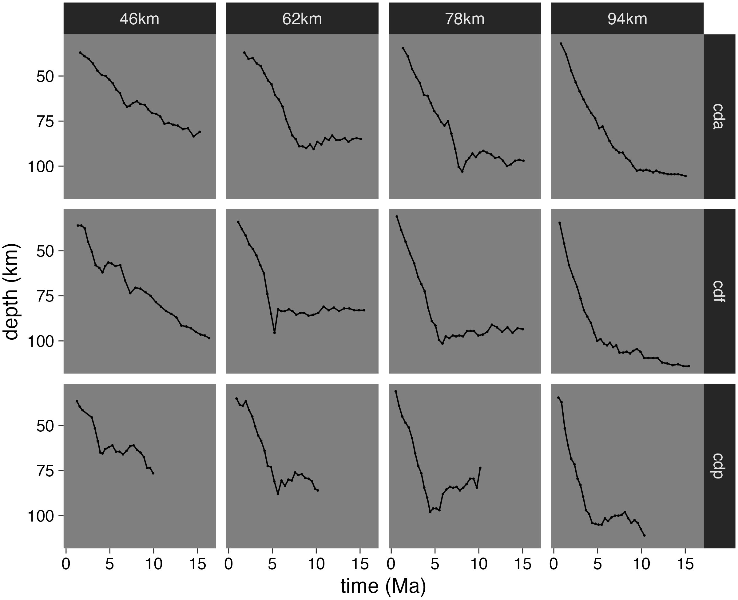
Figure A.1: Serpentine stability depth at the plate interface vs. time for models cda, cdf, and cdp with \(Z_{UP}\) = 46, 62, 78, and 94 km. Serpentine stabilization deepens for approximately 5 Ma of subduction and then remains roughly constant for \(\leq\) 10 Ma. The exceptions are models with very thin \(Z_{UP}\), which exhibit transient behavior for at least 15 Ma. Overall serpentine stability depth after approximately 5 Ma depends on upper-plate thickness.

Numerical experiments in this study suggest a negative dynamic feedback regulating coupling and serpentine dehydration can help explain how similar configurations, in terms of depths to subducting plates beneath arcs (England et al., 2004) and thin upper-plates (Currie & Hyndman, 2006), may occur in subduction zones with different thermo-kinematic boundary conditions and subduction durations. The results indicate that subduction zones quickly (< 5 Ma) develop and stabilize quasi-permanent, generalized configurations with coupling depth dependent on upper-plate thickness.

Notable exceptions occur in models with the thinnest upper-plates (\(Z_{UP}\) = 46 km). Rapid extension due to thin upper-plates form spreading centers in the upper-plate within 5 Ma. Passive asthenospheric upwelling near spreading centers diverts heat from deep within the upper-plate mantle. Enough heat is apparently diverted to disrupt thermal feedbacks regulating coupling and serpentine stability near the plate interface. In principle, diversion of heat from the plate interface could lead to cooler conditions, deeper serpentine stability, and thus deeper coupling. Further testing to confirm this behavior may artificially increase upper-plate strength in thin upper-plate thickness experiments to prevent high rates of spreading.

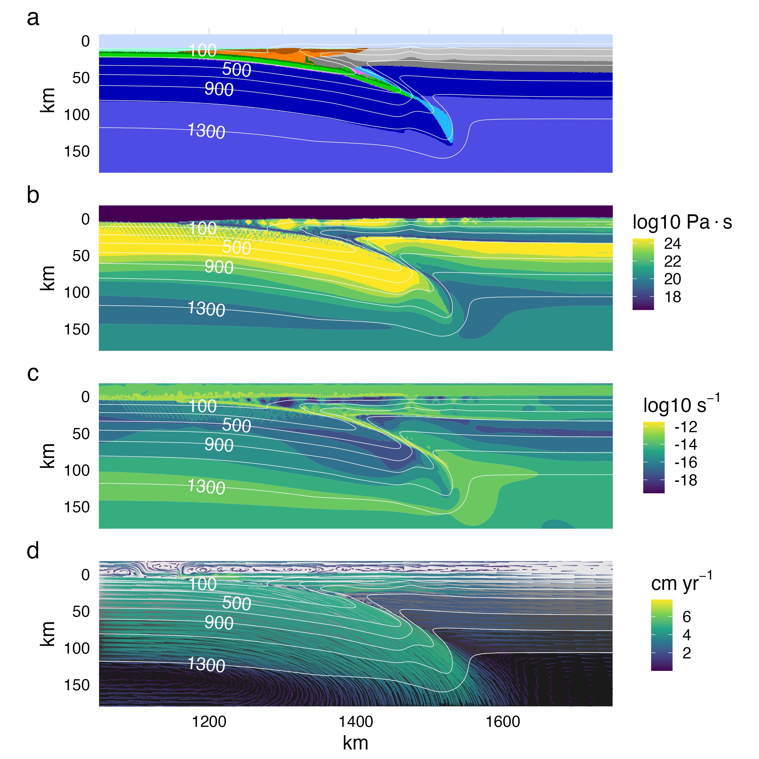
Figure A.2: Visualizing model cdf with \(Z_{UP}\) = 78 km at 1.64 Ma. (a) Rock type. (b) Temperature. (c) Viscosity. (d) Streamlines. Early subduction is facilitated by the prescribed initial weak layer cutting the lithosphere. Strain is localized in the weak serpentine layer along the plate interface. The shallow upper-plate mantle is stagnant and loses heat to the subducting plate, promoting serpentine stabiliization to greater depths. Rock type colors are the same as Figure 2.1.

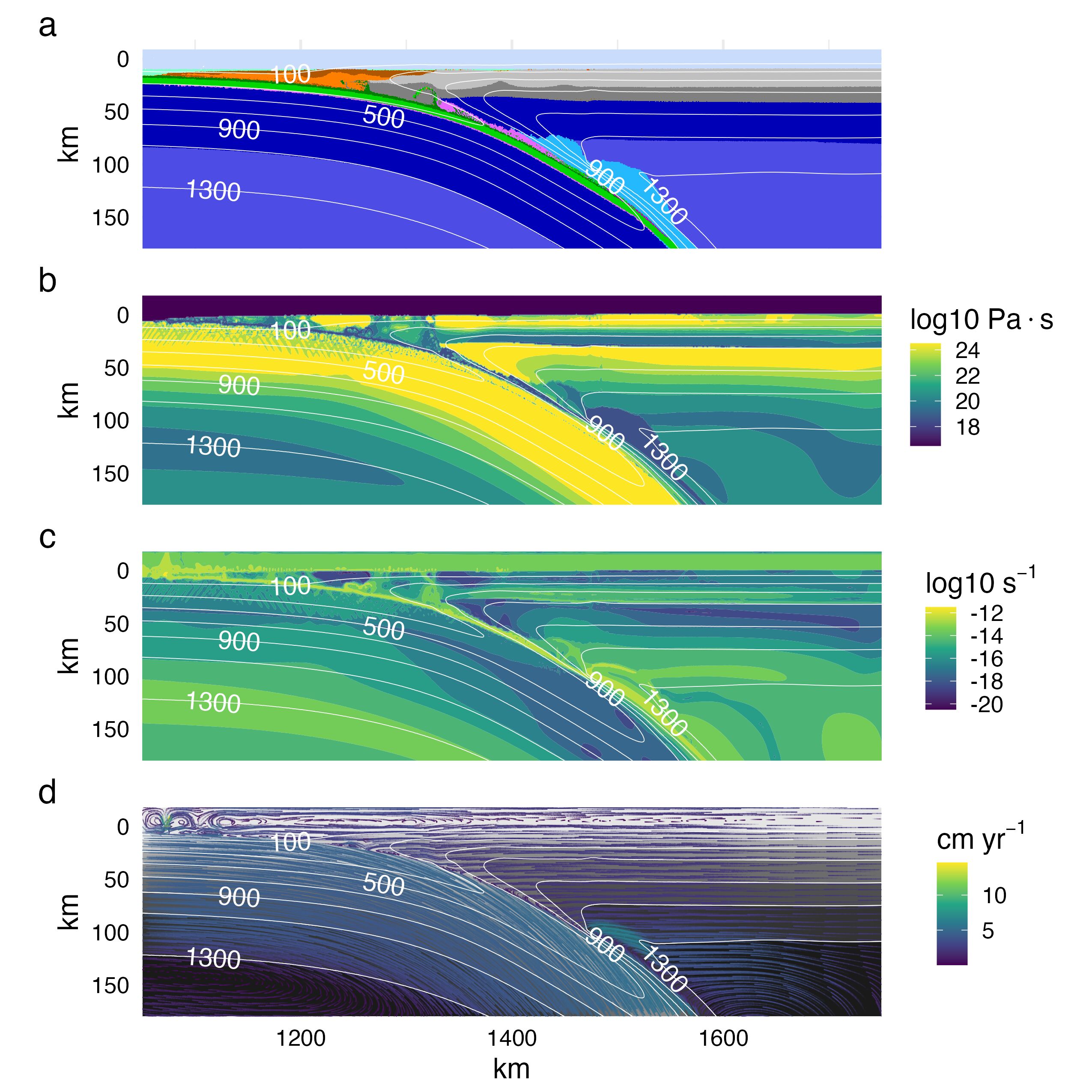
Figure A.3: Visualizing model cdf with \(Z_{UP}\) = 78 km at 5.05 Ma. (a) Rock type. (b) Temperature. (c) Viscosity. (d) Streamlines. By 5 Ma balance is achieved between cooling and heating in the shallow and deep upper-plate mantle, respectively. A feedback regulating heat transfer, serpentine destabilization, and mechanical coupling is already stabilizing coupling depth. Rock type colors are the same as Figure 2.1.

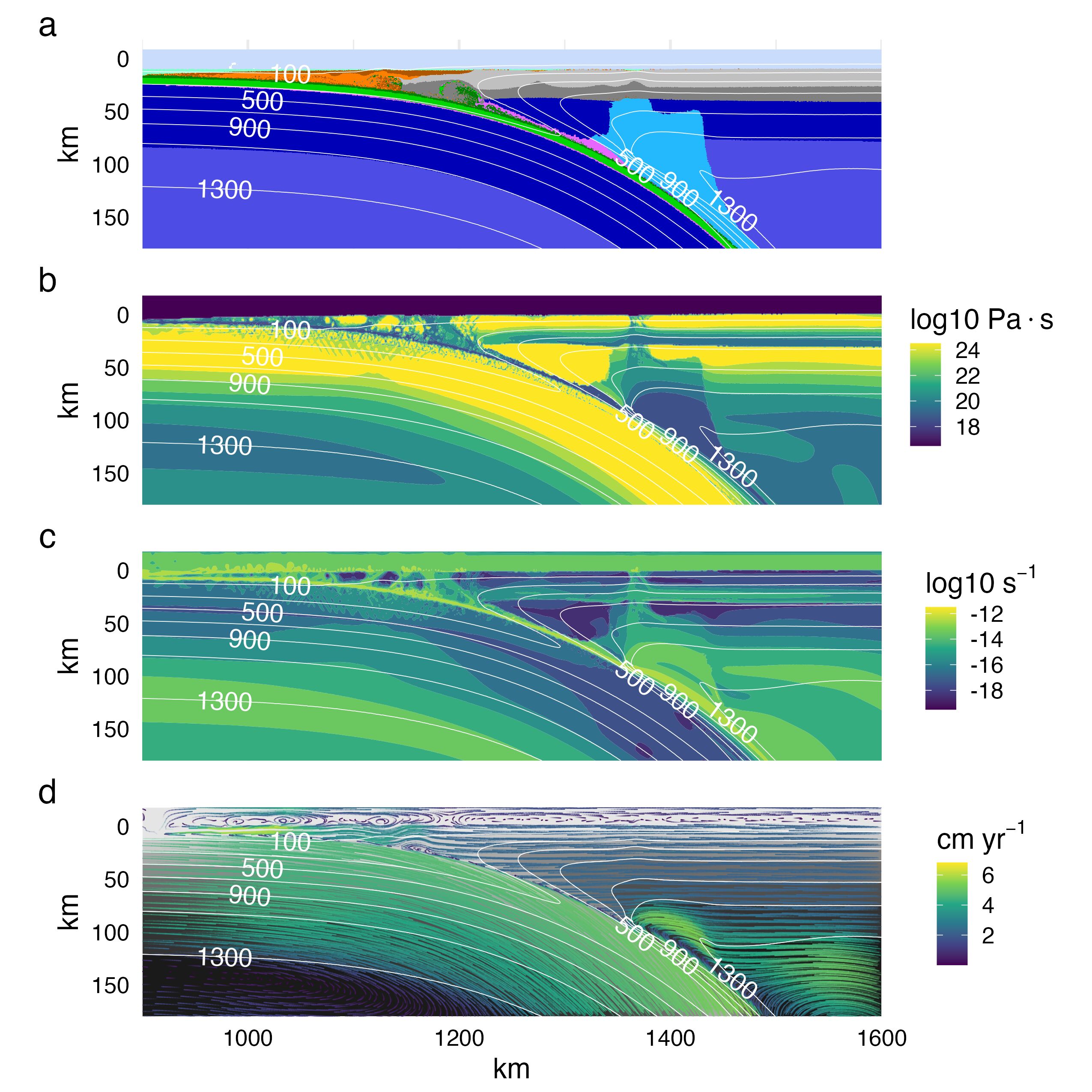
Figure A.4: Visualizing standard model cdf with \(Z_{UP}\) = 78 km at 9.93 Ma. (a) Rock type. (b) Temperature. (c) Viscosity. (d) Streamlines. Geodynamics remain approximately constant from 5 Ma (cf. Figure A.3). The system remains in steady state for as long water fluxes to the upper-plate mantle and serpentine is stable. Rock type colors are the same as Figure 2.1.

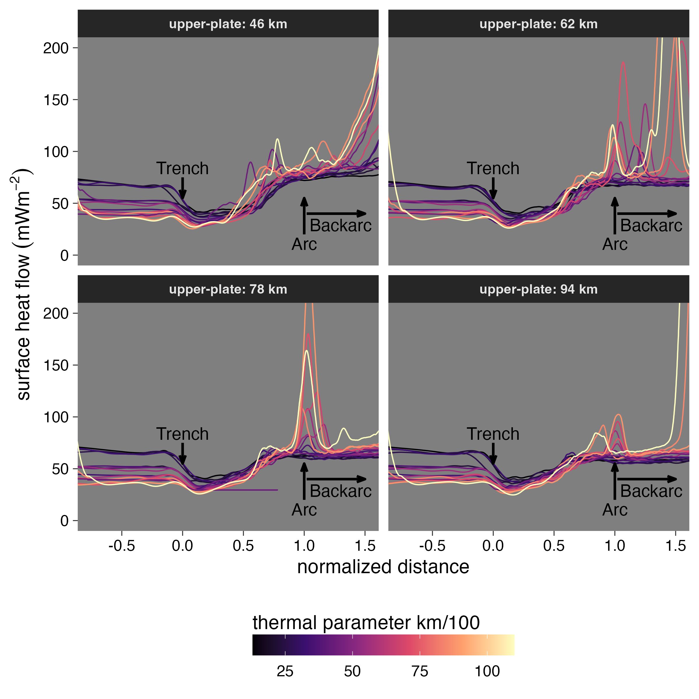
Figure A.5: Surface heat flow calculated at approximately 10 Ma for all numerical experiments. Normalized distance is the distance from the left boundary to the trench, divided by the distance between the trench and arc. Grayscale corresponds to \(\Phi\). High amplitude fluctuations near the arc region (normalized distance = 1.0) correspond to vertical migration of fluids and melts. In the backarc region (normalized distance \(\geq\) 1.0), these fluctuations correspond to lithospheric extension. Backarc extension is most apparent for high-\(\Phi\) experiments (lighter gray lines). Experiments with no extension show a tight distribution of surface heat flow in the backarc region (darker gray lines).

A.2 Regression Summaries

The form of the preferred quadratic regression model in Section 2.3.1 (Figure A.6 & Table A.3) implies a lower limit to coupling depth of approximately 60 km, even for thin upper-plate thickness and, presumably, under warm conditions during nascent subduction. In principle, thin upper-plates could allow effective heat transfer in a flowing shallow asthenospheric mantle—hindering deep stabilization of serpentine. Olivine and pyroxene would be the stable mantle minerals, and strong, shallow coupling between plates would be expected Gerya et al. (2008). However, even the warmest numerical experiments (low-\(\Phi\) & thin upper-plate thickness) in this study eventually stabilize serpentine in the shallow upper-plate mantle. This is evident by increasing depth of mechanical coupling with time for the first 5 Ma of subduction (Figure A.1).

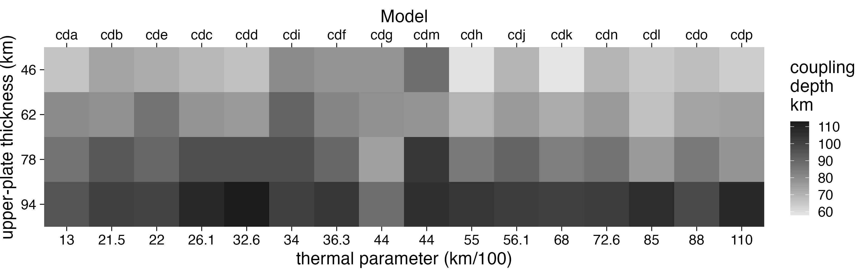
Figure A.6: Coupling depths (\(Z_{cpl}\), grayscale) determined from numerical experiments. Model names are listed along the top axis and correspond to the range of thermal parameter \(\Phi\) values along the bottom axis. Note that the (\(\Phi\)) axis is not linear. \(Z_{cpl}\) increases systematically with increasing \(Z_{UP}\) (change in grayscale down columns) for all models. Trends in \(Z_{cpl}\) with respect to \(\Phi\) (change in grayscale across rows) are less apparent.

Table A.1: Summary of ANOVA test

\(Z_{UP}\) Groups	\(Z_{cpl}\) Estimate	Upper Bound	Lower Bound	p value
	\([km]\)	\([km]\)	\([km]\)
62-46	8.2	2.5	14.0	1.84e-03
78-46	18.0	12.3	23.7	1.08e-10
94-46	33.6	27.8	39.3	1.99e-11
78-62	9.8	4.0	15.5	1.83e-04
94-62	25.3	19.6	31.0	1.99e-11
94-78	15.6	9.8	21.3	7.31e-09
Pair-wise Tukey’s test comparing means between groups. Estimates are differences between means. Null hypothesis is that means are not different

Table A.2: Summary of regression models

Model	Term	Estimate	Std. Error	p value
1	Intercept	89.4	3.7	2.24e-33
1	thermal.parameter	-0.1	0.1	1.55e-01
2	Intercept	36.4	3.2	7.15e-17
2	upper.plate.thickness	0.7	0.0	3.73e-23
3	Intercept	58.9	1.7	1.43e-41
3	upper.plate.thickness^2	0.0	0.0	2.98e-24
4	Intercept	69.2	14.0	6.25e-06
4	upper.plate.thickness	-0.3	0.4	4.63e-01
4	upper.plate.thickness^2	0.0	0.0	1.95e-02
5	Intercept	41.1	3.3	1.14e-18
5	upper.plate.thickness	0.7	0.0	1.12e-24
5	thermal.parameter	-0.1	0.0	1.18e-03
6	Intercept	63.6	2.1	8.29e-39
6	upper.plate.thickness^2	0.0	0.0	5.68e-26
6	thermal.parameter	-0.1	0.0	6.98e-04
7	Intercept	73.8	12.9	3.39e-07
7	upper.plate.thickness	-0.3	0.4	4.23e-01
7	upper.plate.thickness^2	0.0	0.0	1.12e-02
7	thermal.parameter	-0.1	0.0	7.28e-04
models: 1: \(z_c=\phi\), 2: \(z_c=Z_{UP}\), 3: \(z_c=Z_{UP}^2\), 4: \(z_c=Z_{UP}+Z_{UP}^2\), 5: \(z_c=Z_{UP}+\phi\), 6: \(z_c=Z_{UP}^2+\phi\), 7: \(z_c=Z_{UP}+Z_{UP}^2+\phi\)

Table A.3: Coupling depth results

Model	\(Z_{UP}\) \([km]\)	\(\Phi\) \([km/100]\)	\(Z_{cpl}\) \([km]\)
cda	46	13.0	66
cdb	46	21.5	74
cdc	46	26.1	69
cdd	46	32.6	67
cde	46	22.0	72
cdf	46	36.3	78
cdg	46	44.0	78
cdh	46	55.0	59
cdi	46	34.0	80
cdj	46	56.1	70
cdk	46	68.0	58
cdl	46	85.0	65
cdm	46	44.0	79
cdn	46	72.6	70
cdo	46	88.0	68
cdp	46	110.0	64
cda	62	13.0	80
cdb	62	21.5	79
cdc	62	26.1	78
cdd	62	32.6	77
cde	62	22.0	87
cdf	62	36.3	82
cdg	62	44.0	75
cdh	62	55.0	70
cdi	62	34.0	91
cdj	62	56.1	77
cdk	62	68.0	72
cdl	62	85.0	67
cdm	62	44.0	88
cdn	62	72.6	77
cdo	62	88.0	74
cdp	62	110.0	75
cda	78	13.0	87
cdb	78	21.5	94
cdc	78	26.1	97
cdd	78	32.6	97
cde	78	22.0	90
cdf	78	36.3	90
cdg	78	44.0	88
cdh	78	55.0	85
cdi	78	34.0	97
cdj	78	56.1	91
cdk	78	68.0	84
cdl	78	85.0	77
cdm	78	44.0	78
cdn	78	72.6	87
cdo	78	88.0	85
cdp	78	110.0	78
cda	94	13.0	95
cdb	94	21.5	101
cdc	94	26.1	108
cdd	94	32.6	113
cde	94	22.0	100
cdf	94	36.3	104
cdg	94	44.0	104
cdh	94	55.0	104
cdi	94	34.0	101
cdj	94	56.1	102
cdk	94	68.0	101
cdl	94	85.0	107
cdm	94	44.0	106
cdn	94	72.6	102
cdo	94	88.0	98
cdp	94	110.0	108

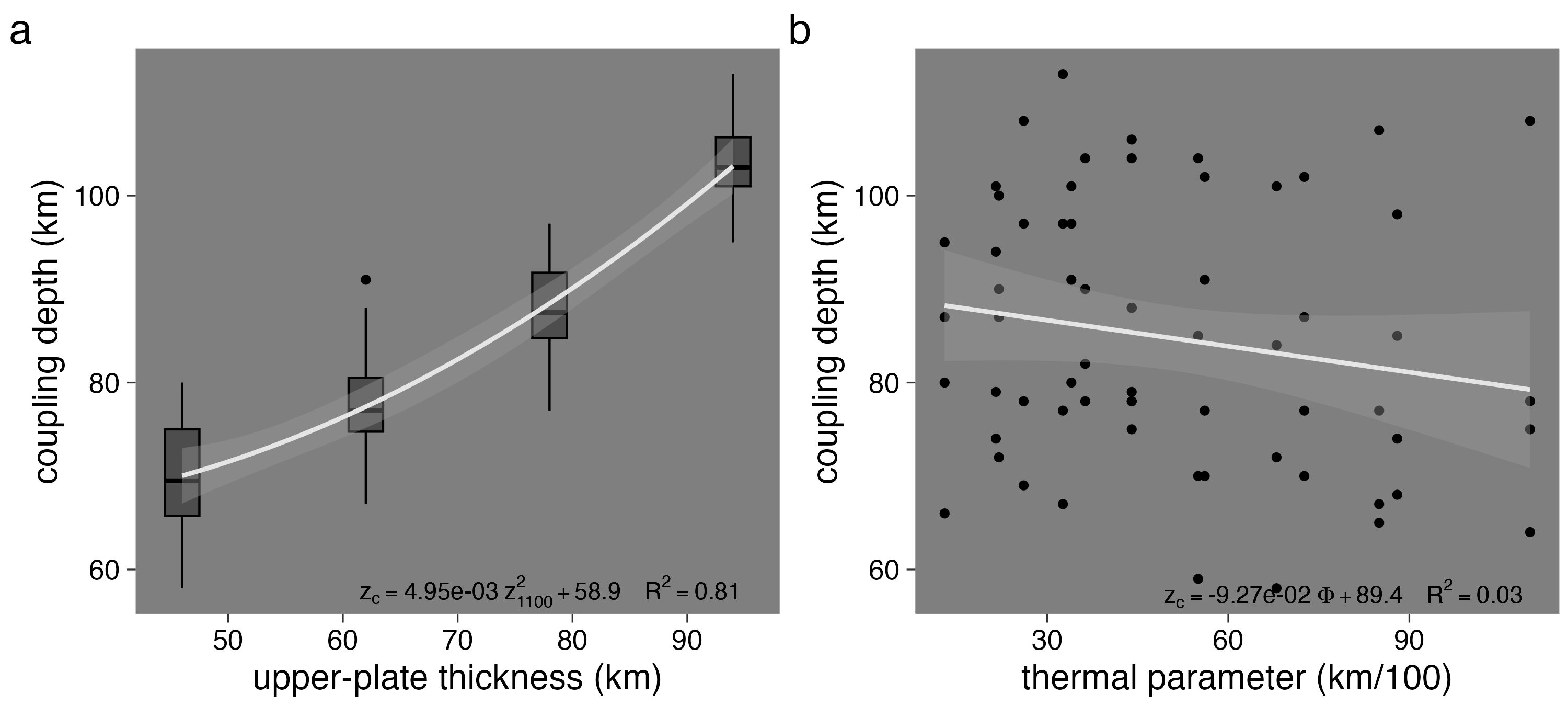
Figure A.7: Bivariate regressions. (a) Coupling depth (\(Z_{cpl}\)) vs. upper-plate thickness (\(Z_{UP}\)) shows \(Z_{cpl}\) increasing approximately quadratically with increasing \(Z_{UP}\). The correlation is highly significant (see Tables A.1 and A.2) and explains more than 80% of the variance in \(Z_{cpl}\). \(Z_{UP}\) alone estimates \(Z_{cpl}\) well. (b) \(Z_{cpl}\) vs. thermal parameter (\(\Phi\)) shows no significant correlation (no line fits with a slope significantly different from zero). \(\Phi\) has little effect on \(Z_{cpl}\) and cannot be used as a standalone estimator.

A.3 (De)hydration Model

The material properties used in the numerical experiments are listed in Table 2.1 and Table A.4. For details about the sedimentation and erosion, melting and extraction, and rheological models, refer to Sizova et al. (2010). Here we discuss only the hydrodynamic model, because it is the most relevant aspect of the numerical experiments.

Hydrodynamics in the numerical models control the timing and magnitude of mantle wedge hydration. The main sources of water delivered to the mantle are altered basaltic crust and seafloor sediments, which we assumed to contain up to 5 \(wt.\% H_{2}O\). We assumed a gradual expulsion of water from pore space and through quasi-continuous dehydration reactions occurring within the slab. Water content is computed using the following equation: \[\begin{equation} \chi_{H_{2}O} = \chi_{H_{2}O_{init}}\times\left(1-\frac{\Delta z}{150\times 10^{3}}\right) \end{equation}\] where \(\chi_{H_{2}O_{init}}\) = 5 \(wt.\%\) and \(\Delta z\) is a marker’s depth below the topographical surface.

If a rock marker dehydrates, an independent water particle is instantaneously generated at the same location with the respective \(H_{2}O\) content. The new water particle is moved in accordance to the local velocity field, described by the following equation: \[\begin{equation} \begin{aligned} \vec{v}_{\text{water}} & = (\vec{v}_x,\ \vec{v}_z) \\ \vec{v}_z & = \vec{v}_z - \vec{v}_{z(\text{percolation})} \\ \end{aligned} \end{equation}\] where \(\vec{v}_{water}\) is the velocity vector of the water particle, \(\vec{v}_{x}\) and \(\vec{v}_{z}\) are the local velocity vectors of the solid state mantle or crust, and \(\vec{v}_{z(percolation)}\) is a imposed constant upward percolation velocity (10 \(cm/year\)). We implicitly neglect kinetics of reactions, as material properties of markers change instantaneously at equilibrium reactions.

Table A.4: Melting curves used in numerical experiments

Material	a	b	c	d	e	f	g	h	i	j
sediments	1200	889	1.79e+04	54	2.02e+04	831	6.00e-02		1262	0.009
felsic crust	1200	889	1.79e+04	54	2.02e+04	831	6.00e-02		1262	0.009
basalt	1600	973	7.04e+05	354	7.78e+07	935	3.50e-03	6.2e-05	1423	0.105
gabbro	1600	973	7.04e+05	354	7.78e+07	935	3.50e-03	6.2e-05	1423	0.105
mantle dry						1394	1.33e-01	-5.1e-05	2073	0.114
mantle hydrated	2400	1240	4.98e+04	323			1.27e+05	3.5e-05	2073	0.114
serpentine	2400	1240	4.98e+04	323			1.27e+05	3.5e-05	2073	0.114
solidus curve: \(T(P)=b+\frac{c}{(P+d)}+\frac{e}{(P+d)^2}\) at $P
liquidus curve: \(T(P) = i+jP\) with \(T\) in \([K]\) and \(P\) in \([MPa]\)
reference: Schmidt & Poli (1998)

A.4 Rheologic Sensitivity Tests on Plate Coupling

Numerical modelling practitioners simulating subduction zones approach mechanical coupling between plates differently. A simple, but highly effective approach, is prescribing a layer of arbitrary strength extending from the surface to an arbitrary depth or temperature along the plate interface. This approach effectively inhibits transfer of shear stress between plates and is analogous to controlling a no-slip condition at the interface (plates move with the same velocity vector beyond the coupling point). Numerous models use this method (e.g. Peacock, 1996; Peacock & Wang, 1999; Syracuse et al., 2010; Wada & Wang, 2009) in part because it allows fine-tuning to specific subduction zone configurations. Serpentine-or talc-rich horizons are typically invoked to justify implementing such a condition at shallow interface depths.

The experiments outlined in Section 2.2 do not explicitly define coupling, but rather use a rheologic model that explicitly follows experimentally determined flow laws and mineral stability fields. This approach conceptually follows and extends petrologic explanations for a weak interface (Hyndman & Peacock, 2003; Peacock & Hyndman, 1999). As a corollary, dehydration of serpentine, or possibly talc, at higher temperatures must strengthen the interface (Agard et al., 2016). Noting that talc is unstable at P > 2.0 GPa in an ultramafic rock (Schmidt & Poli, 1998), a serpentine rheology is arguably the most relevant candidate responsible for a strength increase, and thus coupling, at PT conditions inferred for coupling in active subduction zones (Syracuse et al., 2010; Wada & Wang, 2009).

Sensitivity tests of the rheologic model presented in Section 2.2.2 were run using diverse experiments adjusting the rheology of serpentine (compared to Table 2.1), the shape and position of the antigorite-out reaction (compared to (2.5)), and certain hydrodynamic parameters. For brevity, these results are not presented here. The experiments included:

1. antigorite \(\leftarrow\) wet olivine flow law

2. antigorite and wet olivine \(\leftarrow\) dry olivine flow law

3. isothermal antigorite reaction at 690 ˚C

4. antigorite reaction isothermal Clapeyron slope at 715 ˚C

5. antigorite reaction with positive linear Clapeyron slope

6. linear release of \(H_{2}O\) with depth

7. no fluid-induced weakening

Only experiments 5 and 7 listed above were inconsistent with the results presented Section 2.3. Experiment 5 results in transient coupling depths and discontinuous antigorite stability in the upper-plate mantle, whereas experiment 7 results in two-sided subduction (e.g. Gerya et al., 2008). These sensitivity experiments imply numerical coupling mechanisms are mostly contingent on fluid flux to the upper-plate mantle and the implementation of serpentine stability. The experiments also show coupling is relatively insensitive to the exact flow law parameters.

B A Comparison of Surface Heat Flow Interpolations Near Subduction Zones

B.1 Kriging System and Optimization

B.1.1 Ordinary Kriging

This study applies local isotropic ordinary Kriging methods under the following general assumptions:

• \(\hat{\gamma}(h)\) is directionally invariant (isotropic)

• \(\hat{\gamma}(h)\) is evaluated in two-dimensions and neglects elevation

• The first and second moments of \(Z(u)\) are assumed to follow the conditions:

\[\begin{equation} \begin{aligned} &E[Z(u)] = \hat{Z}(u) = constant \\ &E[(Z(u + h) - \hat{Z}(u))(Z(u) - \hat{Z}(u))] = C(h) \end{aligned} \tag{B.1} \end{equation}\] where \(h\) is the lag distance, \(C(h)\) is the covariance function, \(E[Z(u)]\) is the expected value of the random variable \(Z(u)\), and \(\hat{Z}(u)\) is the arithmetic mean of \(Z(u)\).

Equation (B.1) is known as “weak second-order stationarity”. It assumes the underlying probability distribution of the observations \(Z(u)\) does not change in space and the covariance \(C(h)\) only depends on the distance \(h\) between two observations. These assumptions are expected to be valid in cases where the underlying natural process is stochastic, spatially continuous, and has the property of additivity such that \(\frac{1}{n}\sum_{i=1}^n Z(u_i)\) has the same meaning as \(Z(u)\) (Bárdossy, 1997).

The following are two illustrative cases where Equation (B.1) is likely valid:

The thickness of a sedimentary unit with a homogeneous concentration of radioactive elements can be approximated by \(q_s = q_b + \int A \,dz\), where \(q_b\) is a constant heat flux entering the bottom of the layer and \(A\) is the heat production within the layer with thickness \(z\) (Furlong & Chapman, 2013). If one has two samples, \(Z(u_1)\) = 31 mW/m\(^2\) and \(Z(u_2)\) = 30.5 mW/m\(^2\), their corresponding thicknesses would be \(Z'(u_1)\) = 1000 m and \(Z'(u_2)\) = 500 m for \(A\) = 0.001 mW/m\(^3\) and \(q_b\) = 30 mW/m\(^2\). The variable, \(Z(u)\), in this case is additive because the arithmetic mean of the samples is a good approximation of the average sedimentary layer thickness, \((Z(u_1) + Z(u_2)) /\) 2 = 750 m.

The age of young oceanic lithosphere can be approximated by \(q_s(t) = kT_b(\pi\kappa t)^{-1/2}\), where \(q_s(t)\) is surface heat flow of a plate with age, \(t\), \(T_b\) is the temperature at the base of the plate, \(k\) is thermal conductivity, and \(\kappa = k/\rho C_p\) is thermal diffusivity (Stein & Stein, 1992). Using reasonable values for \(k\) = 3.138 W/mK, \(\rho\) = 3330 kg/m\(^3\), \(C_p\) = 1171 J/kgK, \(T_b\) = 1350 ˚C, two samples, \(Z(u_1)\) = 180 mW/m\(^2\) and \(Z(u_2)\) = 190 mW/m\(^2\), would correspond to plates with ages of \(Z'(u_1)\) = 10 Ma, and \(Z'(u_2)\) = 9 Ma, respectively. Since \(Z(u_1) + Z(u_2) /\) 2 = 185 mW/m\(^2\) and \(Z'(185~mW/m^2)\) = 9.5 Ma = \(Z'(u_1) + Z'(u_2) /\) 2, the variable \(Z(u)\) in this case is also additive.

Equation (B.1) is likely invalid in regions that transition among two or more tectonic regimes, however. For example, the expected (mean) heat flow \(E[Z(u)]\) will change when moving from a spreading center to a subduction zone and thus \(E[Z(u)] \neq constant\) over the region of interest. In other words, stationarity is violated and Kriging estimates may become spurious. Careful selection of Kriging parameters (outlined below; e.g. maximum point-pairs to use for local Kriging) can reduce or eliminate violations of stationarity assumptions embodied in (B.1).

The second step is fitting a variogram model \(\gamma(h)\) to the experimental variogram. This study fits six popular variogram models with sills (or theoretical sills) to the experimental variogram. The models are defined as (Pebesma, 2004): \[\begin{equation} \begin{aligned} Bes &\leftarrow \gamma(h) = 1 - \frac{h}{a}\ K_1\left(\frac{h}{a}\right) \quad \text{for } \ h \geq 0 \\ Cir &\leftarrow \gamma(h) = \begin{cases} \frac{2}{\pi}\frac{h}{a}\ \sqrt{1-\left(\frac{h}{a}\right)^2} + \frac{2}{\pi}\ arcsin\left(\frac{h}{a}\right) \quad \text{for } \ 0 \leq h \leq a \\ nug + sill \quad \text{for } \ h > a \end{cases} \\ Exp &\leftarrow \gamma(h) = 1 - exp\left(\frac{-h}{a}\right) \quad \text{for } \ h \geq 0 \\ Gau &\leftarrow \gamma(h) = 1 - exp\left(\left[\frac{-h}{a}\right]^2\right) \quad \text{for } \ h \geq 0 \\ Lin &\leftarrow \gamma(h) = \begin{cases} \frac{h}{a} \quad \text{for } \ 0 \leq h \leq a \\ nug + sill \quad \text{for } \ h > a \end{cases} \\ Sph &\leftarrow \gamma(h) = \begin{cases} \frac{3}{2}\frac{h}{a} - \frac{1}{2}\left(\frac{h}{a}\right)^3 \quad \text{for } \ 0 \leq h \leq a \\ nug + sill \quad \text{for } \ h > a \end{cases} \\ \end{aligned} \tag{B.2} \end{equation}\] where \(h\) is the lag distance, \(nug\) is the nugget, \(sill\) is the sill, \(a\) is the effective range, \(K_1\) is a modified Bessel function. The models are Bessel, Circular, Exponential, Gaussian, Linear, and Spherical. For models without explicit sills (Bes, Exp, Gau), the effective range \(a\) is the distance where the variogram reaches 95% of its maximum defined as 4\(a\), 3\(a\), and \(\sqrt{3}a\) for Bes, Exp, and Gau, respectively (Gräler et al., 2016; Pebesma, 2004). The function fit.variogram in gstat is used to try all variogram models. The best model is selected by the minimum weighted least squares (Pebesma, 2004) error with weights proportional to the number of points in each lag divided by the squared lag distance \(wt = N(h)_k/h_k^2\). Gaussian models produce spurious results in every case and are not included in the final analysis. Moreover, Circular models produce indistinguishable results from Spherical models, and so too were omitted from the final analysis.

Ordinary Kriging is used for interpolation, which estimates unknown observations \(\hat{Z}(u)\) as a linear combination of all known observations (Bárdossy, 1997): \[\begin{equation} \hat{Z}(u) = \sum_{i=1}^n \lambda_i Z(u_i) \tag{B.3} \end{equation}\]

The conditions in Equation (B.1) set up a constrained minimization problem that can be solved with a system of linear equations. The expected value of \(Z(u)\) is assumed to be the mean according to (B.1), so the weights must be: \[\begin{equation} \begin{aligned} E[\hat{Z}(u)] &= \sum_{i=1}^n \lambda_i E[Z(u_i)] \\ \sum_{i=1}^n \lambda_i &= 1 \end{aligned} \tag{B.4} \end{equation}\]

This constraint is known as the unbiased condition, which states that the sum of the weights must equal one. However, there is an infinite set of real numbers one could use for the weights, \(\lambda_i\). The goal is to find the set of weights in Equation (B.3) that minimizes the estimation variance. This can be solved by minimizing the covariance function, \(C(h)\) from Equation (B.1): \[\begin{equation} \begin{aligned} & \sigma^2(u) = Var[Z(u) - \hat{Z}(u)] = \\ & E\left[(Z(u) - \sum_{i=1}^n \lambda_i Z(u_i))^2\right] = \\ & E\left[Z(u)^2 + \sum_{j=1}^n \sum_{i=1}^n \lambda_j \lambda_i Z(u_j)Z(u_i) - 2 \sum_{i=1}^n \lambda_i Z(u_i)Z(u)\right] = \\ & C(0) + \sum_{j=1}^n \sum_{i=1}^n \lambda_j \lambda_i C(u_i - u_j) - 2 \sum_{i=1}^n \lambda_i C(u_i - u) \end{aligned} \tag{B.5} \end{equation}\]

Minimizing Equation (B.5) with respect to the unbiased condition (Equation (B.4)), yields the best linear unbiased estimator (BLUE, Bárdossy, 1997) for Equation (B.3) and together comprise the Kriging system of equations. The functions krige and krige.cv in gstat are used for surface heat flow interpolation and error estimation by k-fold cross-validation (Pebesma, 2004).

B.1.2 Optimization with nloptr

Achieving accurate Kriging results depends on one’s choice of many Kriging parameters, \(\Theta\). In this study, we investigate a set of parameters: \[\begin{equation} \Theta = \{model,\ n_{lag},\ cut,\ n_{max},\ shift\} \tag{B.6} \end{equation}\] where \(model\) is one of the variogram models defined in Equation (B.2), \(n_{lag}\) is the number of lags, \(cut\) is a lag cutoff proportionality constant, \(n_{max}\) is the maximum point-pairs for local Kriging, and \(shift\) is a horizontal lag shift constant. The lag cutoff constant \(cut\) controls the maximum separation distance between pairs of points used to calculate the experimental variogram (i.e. the x-axis range or “width” of the experimental variogram). The horizontal lag shift constant \(shift\) removes the first few lags from being evaluated by effectively shifting all lags to the left proportionally by \(shift\). This is necessary to avoid negative ranges when fitting experimental variograms with anomalously high variances at small lag distances.

The goal is to find \(\Theta\) such that the Kriging function \(f(x_i;\ \Theta)\) gives the minimum error defined by a cost function \(C(\Theta)\), which represents the overall goodness of fit of the interpolation. This study defines a cost function that simultaneously considers errors between the experimental variogram \(\hat{\gamma}(h)\) and modelled variogram \(\gamma(h)\), and between surface heat flow observations \(Z(u_i)\) and Kriging estimates \(\hat{Z}(u)\) (after Li et al., 2018): \[\begin{equation} \begin{aligned} C(\Theta) &= w_{vgrm}\ C_{vgrm}(\Theta) + w_{interp}\ C_{interp}(\Theta) \\ &w_{vgrm} + w_{interp} = 1 \end{aligned} \tag{B.7} \end{equation}\] where \(C_{vgrm}(\Theta)\) is the normalized RMSE evaluated during variogram fitting and \(C_{interp}(\Theta)\) is the normalized RMSE evaluated during Kriging. Weighted ordinary least squares is used to evaluate \(C_{vgrm}(\Theta)\), whereas k-fold cross-validation is used to evaluate \(C_{interp}(\Theta)\). K-fold splits the dataset \(|Z(u_i)|\) into \(k\) equal intervals, removes observations from an interval, and then estimates the removed observations by fitting a variogram model to data in the remaining \(k-1\) intervals. This process is repeated over all \(k\) intervals so that the whole dataset has been cross-validated. The final expression to minimize becomes: \[\begin{equation} \begin{aligned} &C(\Theta) = \\ &\frac{w_{vgrm}}{\sigma_{vgrm}}\ \left(\frac{1}{N(h)}\ \sum_{k=1}^{N}\ w(h_k)\ [\hat{\gamma}(h_k)-\gamma(h_k;\ \Theta)]^2\right)^{1/4} + \\ &\frac{w_{interp}}{\sigma_{interp}}\ \left(\frac{1}{M}\ \sum_{i=1}^{M}\ [Z(u_i)-\hat{Z}(u_i;\ \Theta)]^2\right)^{1/2} \end{aligned} \tag{B.8} \end{equation}\] where \(N(h)\) is the number of point-pairs used to evaluate the experimental variogram and \(w(h_k) = N(h)_k/h_k^2\) are weights defining the importance of the \(kth\) lag on the variogram model fit. \(Z(u_i)\) and \(\hat{Z}(u_i;\ \Theta)\) are the observed and estimated values, respectively, and m is the number of measurements in \(|Z(u_i)|\). The RMSEs are normalized by dividing by \(\sigma_{vgrm}\) and \(\sigma_{interp}\), which represent the standard deviation of the experimental variogram \(\hat{\gamma}(h)\) and surface heat flow observations \(Z(u_i)\), respectively. The weights \(w_{vgrm}\) and \(w_{interp}\) were varied between 0 and 1 to test the effects on \(C(\Theta)\). Preferred weights of \(w_{vgrm}\) = \(w_{interp}\) = 0.5 are selected to balance the effects of \(C_{vgrm}(\Theta)\) and \(C_{interp}(\Theta)\) on the cost function.

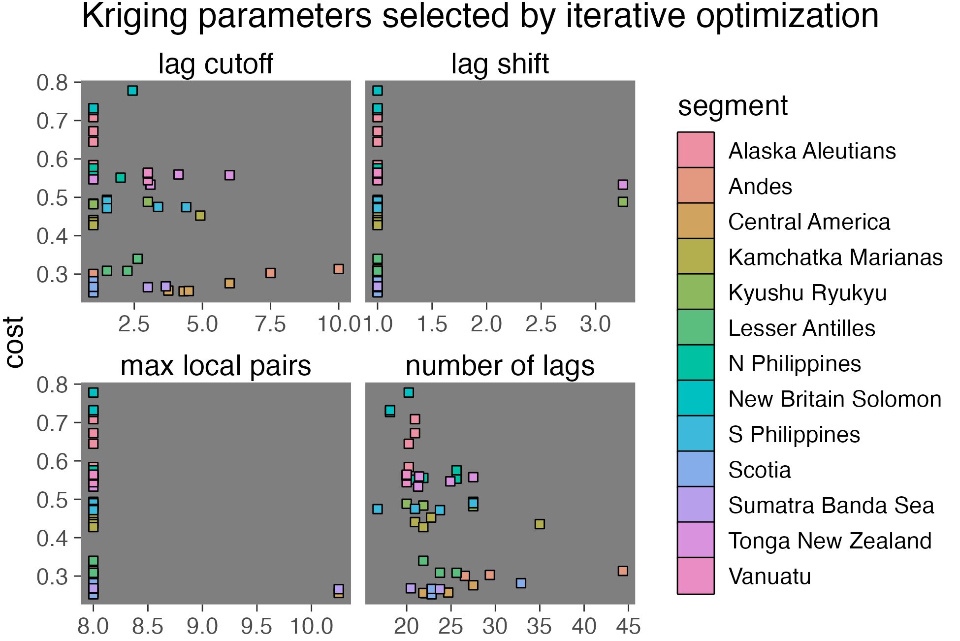
Figure B.1: Summary of optimized Kriging parameters. Cost does not correlate strongly with most Kriging parameters (solid black line with ivory 95% confidence intervals), indicating the optimization procedure is successfully generalizable across subduction zone segments. The exception is a correlation between cost and the logarithm of the experimental variogram sill. Note that parameter values adjust from an initial value (solid white line) during the optimization procedure.

Minimization of \(C(\Theta)\) is achieved by non-linear constrained optimization using algorithms defined in the R package nloptr (Ypma, 2014). Global search methods had limited success compared to local search methods. See the official documentation for more information on nloptr and available optimization algorithms. The run used to produce the visualizations in this study apply the NLOPT_LN_COBYLA method (constrained optimization by linear approximation, Powell, 1994) with 50 max iterations, leave-one-out cross-validation (k-fold \(=\) the number of observations) in the evaluated segment, and cost function weights of \(w_{vgrm}\) = \(w_{interp}\) = 0.5 (Figure B.2). All data, code, and instructions to reproduce results in this study can be found on GitHub at https://github.com/buchanankerswell/kerswell_kohn_backarc.

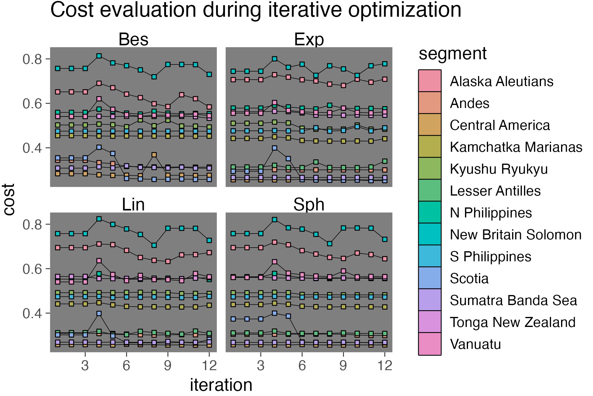
Figure B.2: Cost function minimization for Kriging interpolations. Most variogram models (panels) converge on a local optimum for most Kriging domains (lines) after 15-20 iterations. Each line represents one of thirteen subduction zone segments. See text for bound constraints and other options passed to the optimization procedure.

B.2 Variogram Models

Fitted variograms for Alaska Aleutians

Fitted variograms for Andes

Fitted variograms for Central America

Fitted variograms for Kamchatka Marianas

Fitted variograms for Kyushu Ryukyu

Fitted variograms for Lesser Antilles

Fitted variograms for N Philippines

Fitted variograms for New Britain Solomon

Fitted variograms for S Philippines

Fitted variograms for Scotia

Fitted variograms for Sumatra Banda Sea

Fitted variograms for Tonga New Zealand

Fitted variograms for Vanuatu

Table B.1: Optimum variogram models and Kriging accuracy

Segment	Model	Cutoff	Lags	Shift	\(n_{max}\)	Sill	Range	Cost	\(RMSE_K\)
						\((mWm^{-2})^2\)	km	mW/m\(^2\)	mW/m\(^2\)
Alaska Aleutians	Bes	1.0	16.3	1.0	8.4	841	77	0.498	74.6
Alaska Aleutians	Exp	1.0	15.0	1.9	5.0	837	111	0.665	14.2
Alaska Aleutians	Lin	3.0	20.6	3.4	8.0	790	243	0.621	15.1
Alaska Aleutians	Sph	2.4	19.1	5.3	6.4	818	734	0.629	14.5
Andes	Bes	8.7	26.5	2.1	6.2	2566	5	0.312	38.0
Andes	Exp	1.6	20.8	8.5	12.4	4631	165	0.294	34.9
Andes	Lin	3.6	24.8	5.0	11.8	6084	933	0.297	38.7
Andes	Sph	2.8	18.2	5.3	11.6	5457	558	0.296	35.0
Central America	Bes	5.3	30.4	1.0	11.9	2085	4	0.267	40.4
Central America	Exp	4.9	21.2	3.9	12.4	4683	265	0.248	33.4
Central America	Lin	5.1	27.1	1.0	7.7	2218	14	0.253	35.4
Central America	Sph	6.2	27.2	4.0	13.1	2926	271	0.251	33.0
Kamchatka Marianas	Bes	3.9	25.1	1.0	11.0	1713	10	0.449	36.4
Kamchatka Marianas	Exp	1.0	18.9	1.0	8.4	1783	64	0.428	30.5
Kamchatka Marianas	Lin	1.0	22.2	6.0	6.4	1797	1528	0.424	31.2
Kamchatka Marianas	Sph	1.7	18.5	7.5	6.9	1787	1355	0.424	31.2
Kyushu Ryukyu	Bes	2.4	20.4	1.8	5.9	1843	3	0.491	33.4
Kyushu Ryukyu	Exp	2.4	21.4	5.8	7.8	1898	34	0.487	33.3
Kyushu Ryukyu	Lin	3.2	19.8	3.3	8.3	1898	183	0.487	37.8
Kyushu Ryukyu	Sph	3.0	20.0	3.3	8.1	1903	216	0.488	34.2
Lesser Antilles	Bes	2.0	18.3	2.5	7.2	554	13	0.329	20.9
Lesser Antilles	Exp	1.5	25.1	1.4	10.5	657	68	0.309	12.4
Lesser Antilles	Lin	1.5	24.2	1.1	11.0	653	77	0.297	13.3
Lesser Antilles	Sph	2.7	24.2	3.3	10.2	582	122	0.306	12.6
N Philippines	Bes	1.4	18.3	1.0	7.9	1258	19	0.548	32.0
N Philippines	Exp	2.1	15.0	1.3	5.9	1266	25	0.567	26.7
N Philippines	Lin	3.0	20.0	1.0	8.6	1310	40	0.552	27.3
N Philippines	Sph	1.0	17.8	4.2	8.6	946	516	0.550	27.3
New Britain Solomon	Bes	3.9	20.6	3.5	10.2	744	61	0.694	6.8
New Britain Solomon	Exp	1.6	16.1	1.0	7.4	723	68	0.732	8.0
New Britain Solomon	Lin	2.0	20.2	5.1	10.2	693	228	0.609	28.2
New Britain Solomon	Sph	1.2	18.7	3.6	10.1	694	320	0.657	7.0
S Philippines	Bes	4.1	16.5	1.1	5.3	1086	20	0.465	33.9
S Philippines	Exp	1.3	19.0	2.0	5.7	1227	271	0.466	21.9
S Philippines	Lin	3.2	29.0	1.0	5.0	1014	40	0.464	22.9
S Philippines	Sph	1.3	28.2	8.0	5.3	1056	578	0.466	21.9
Scotia	Bes	3.1	20.7	3.2	10.0	2120	195	0.247
Scotia	Exp	2.6	15.6	4.4	7.9	4503	1148	0.230	10.9
Scotia	Lin	3.0	23.8	3.2	8.0	1876	563	0.243	10.9
Scotia	Sph	2.7	20.8	4.8	7.9	3655	1766	0.228	10.9
Sumatra Banda Sea	Bes	3.2	20.1	1.2	10.3	1604	63	0.307
Sumatra Banda Sea	Exp	3.1	24.1	1.0	10.6	2128	245	0.267	19.4
Sumatra Banda Sea	Lin	6.6	23.0	5.8	12.1	4199	1547	0.266	20.4
Sumatra Banda Sea	Sph	6.6	21.0	5.1	12.8	10598	5850	0.266	20.4
Tonga New Zealand	Bes	5.6	17.2	7.0	7.5	1566	186	0.531	40.7
Tonga New Zealand	Exp	1.0	18.9	8.6	6.3	2072	1657	0.533	20.8
Tonga New Zealand	Lin	3.7	24.9	3.6	10.1	1293	321	0.521	23.8
Tonga New Zealand	Sph	4.9	23.7	5.5	7.4	1307	436	0.534	19.9
Vanuatu	Bes	3.0	20.5	3.6	10.3	3101	113	0.518	59.5
Vanuatu	Exp	3.0	19.8	3.4	8.3	3188	197	0.549	17.8
Vanuatu	Lin	1.2	20.4	2.6	10.8	2918	286	0.517	54.6
Vanuatu	Sph	1.4	17.9	3.3	7.3	2970	468	0.537	17.5
key: \(n_{max}\): max point-pairs, \(RMSE_K\): Kriging accuracy

B.3 ThermoGlobe Summary

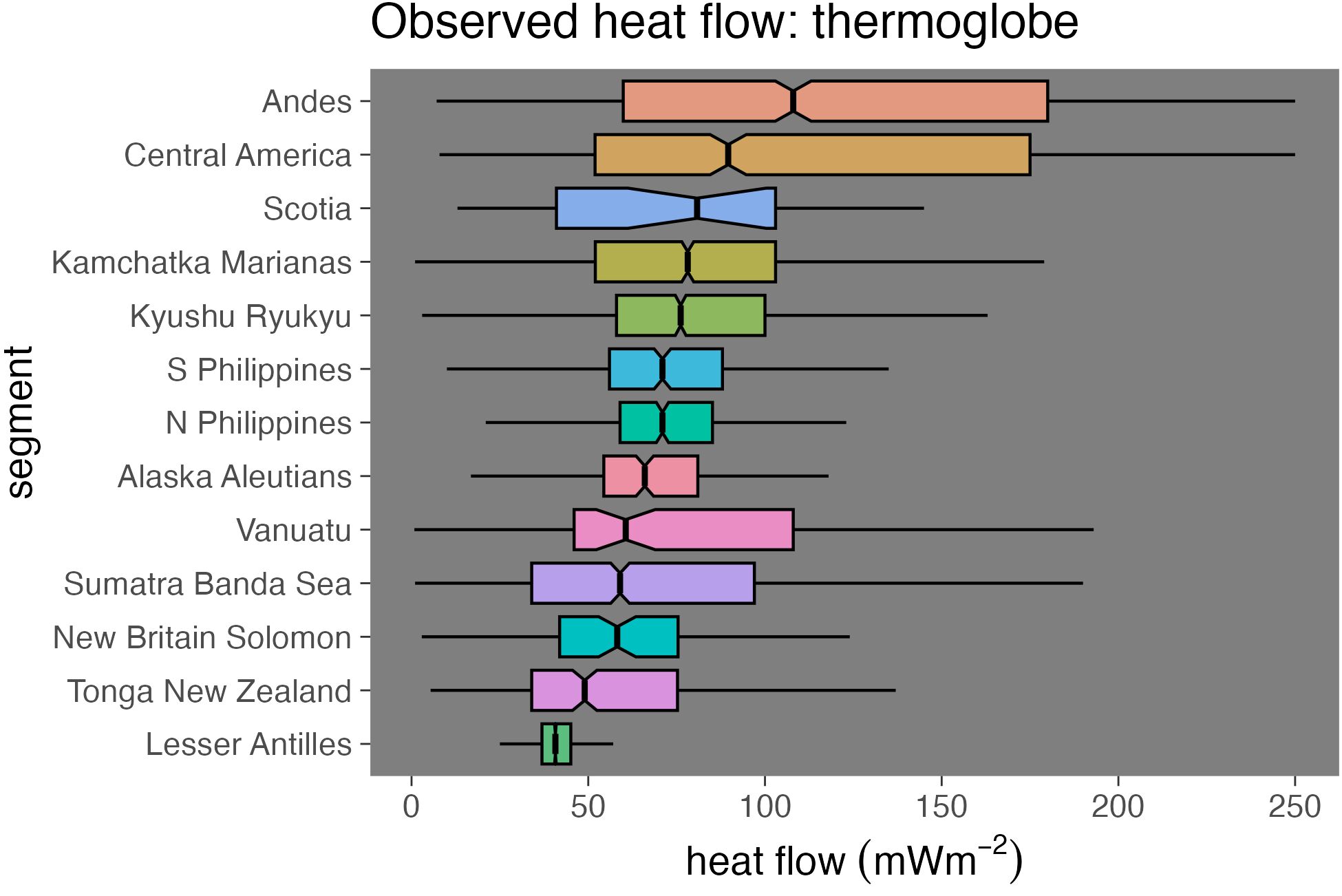
Figure B.3: Distribution of ThermoGlobe observations from Lucazeau (2019) cropped within 1000 km-radius buffers around 13 active subduction zone segments. Heat flow distributions are centered between 41 and 108 mW/m\(^2\), generally right-skewed, and irregularly distributed. Skewness reflects near-surface perturbations from geothermal systems and tectonic regions with high thermal activity while irregularity reflects complex heat exchange acting across multiple spatial scales from 10\(^-1\) to 10\(^3\) km.

Table B.2: ThermoGlobe heat flow summary

Segment	n	Min	Max	Median	IQR	Mean	\(\sigma\)
Alaska Aleutians	290	6	196	66	27	71	28
Andes	1398	7	250	108	120	119	66
Central America	1441	8	250	89	123	110	67
Kamchatka Marianas	2268	1	248	78	51	83	42
Kyushu Ryukyu	1895	3	250	76	42	84	42
Lesser Antilles	3008	13	242	41	8	46	18
N Philippines	569	3	231	71	26	75	33
New Britain Solomon	100	3	143	58	34	61	26
S Philippines	458	1	224	71	32	74	33
Scotia	25	13	145	81	62	79	43
Sumatra Banda Sea	1415	1	247	59	63	67	42
Tonga New Zealand	356	5	218	49	41	60	37
Vanuatu	137	1	223	61	62	80	52
key: n: [# of observations], all other units are in mW/m\(^2\)
note: ThermoGlobe data are filtered for quality, restricted to [0, 250) mW/m\(^2\), and cropped within 1000 km-radius buffers of segment boundaries

B.4 Comparing Similarity and Kriging Interpolations

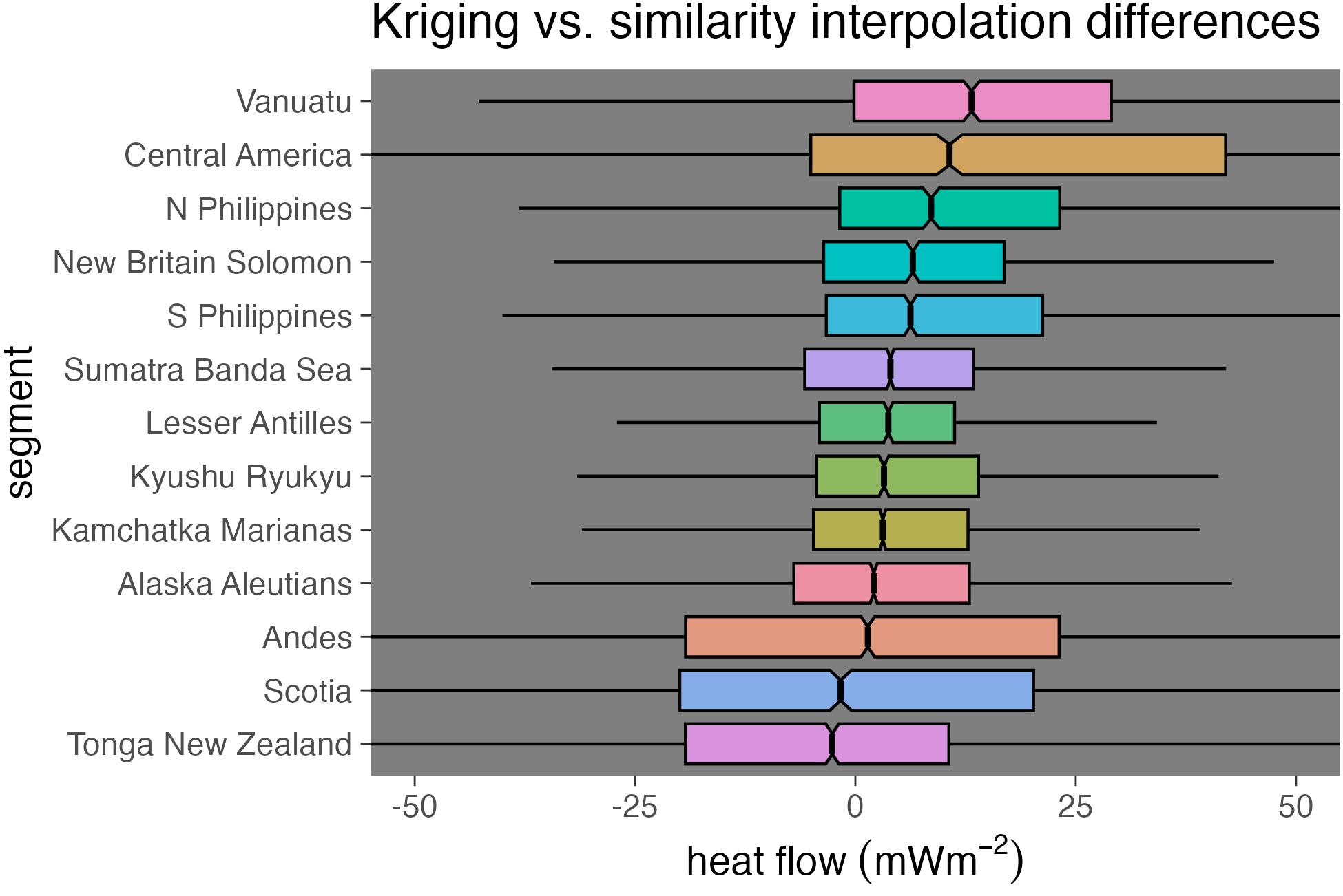
Figure B.4: Differences between Similarity and Kriging interpolations by segment, computed as Similarity-Kriging. Differences are centered near zero with medians ranging from -1 to 14 mW/m\(^2\), but broadly distributed with IQRs from 15 to 50 mW/m\(^2\) and some long tails extending from -1000 to 205 mW/m\(^2\). Positive medians and right skew indicate a general tendency towards higher surface heat flow predictions by Similarity compared to Kriging. The broadest distributions (Andes and Central America) reflect less subtle differences between methods. Distributions are colored by quartiles (25%, 50%, 75%). Similarity interpolation from Lucazeau (2019).

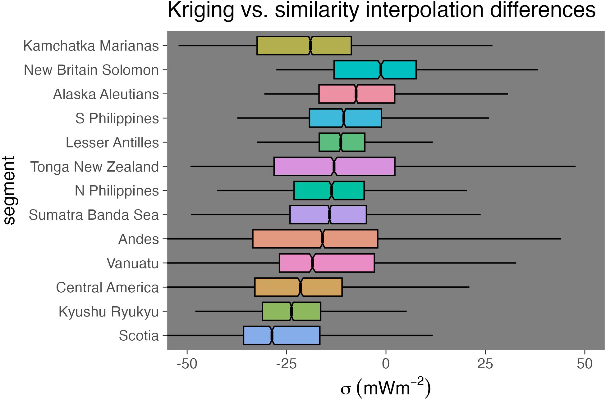
Figure B.5: Summary of differences between Similarity and Kriging uncertainties computed as Similarity-Kriging. Differences are centered at slightly negative values with median differences ranging from -23 to -3 mW/m\(^2\), and relatively narrowly distributed with IQRs from 4 to 13 mW/m\(^2\) and some long tails extending from -50 to 70 mW/m\(^2\). Negative medians indicate greater uncertainties by Kriging compared to Similarity. Distributions are colored by quantiles (25%, 50%, 75%). Similarity data from Lucazeau (2019). Refer to Figure B.4 for estimate differences.

Table B.3: Summary of Similarity-Kriging prediction differences

Segment	Min	Max	Median	IQR	Mean	\(\sigma\)
Alaska Aleutians	-1000	126	2	22	-1	43
Andes	-124	169	0	41	0	33
Central America	-128	205	12	50	20	42
Kamchatka Marianas	-144	178	4	18	6	23
Kyushu Ryukyu	-123	167	4	21	6	23
Lesser Antilles	-129	106	4	15	2	21
N Philippines	-144	141	8	25	11	22
New Britain Solomon	-70	169	7	21	10	22
S Philippines	-79	189	6	25	9	23
Scotia	-126	199	3	40	4	34
Sumatra Banda Sea	-153	144	3	21	2	22
Tonga New Zealand	-142	188	-1	24	0	27
Vanuatu	-147	204	14	31	13	34
note: All units are mW/m\(^2\)

Table B.4: Summary of Similarity-Kriging uncertainty differences

Segment	Model	Min	Max	Median	IQR	Mean	\(\sigma\)
Alaska Aleutians	Bes	-24	45	-3	7	-2	8
Andes	Exp	-46	46	-23	12	-22	11
Central America	Exp	-50	57	-20	12	-20	13
Kamchatka Marianas	Sph	-21	70	-3	6	-1	8
Kyushu Ryukyu	Lin	-43	33	-11	7	-10	7
Lesser Antilles	Lin	-27	18	-12	8	-12	6
N Philippines	Bes	-38	29	-21	13	-21	10
New Britain Solomon	Lin	-12	19	-7	5	-4	7
S Philippines	Lin	-38	0	-23	11	-23	7
Scotia	Sph	-11	3	-7	4	-6	4
Sumatra Banda Sea	Sph	-36	40	-4	6	-2	8
Tonga New Zealand	Lin	-15	59	-5	7	-1	12
Vanuatu	Lin	-24	36	-11	10	-7	13
note: Showing optimal Kriging models only, difference is calculated as Similarity-Kriging
key: Cost: [mW/m\(^2\)], n: number of target locations (grid size), all other units are mW/m\(^2\)

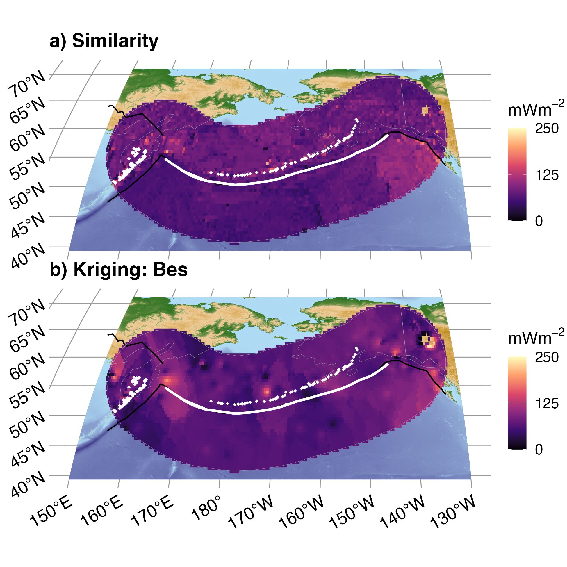
Figure B.6: Similarity (a) and Kriging (b) interpolations for Alaska Aleutians. Refer to the main text for explanation of panels and colors.

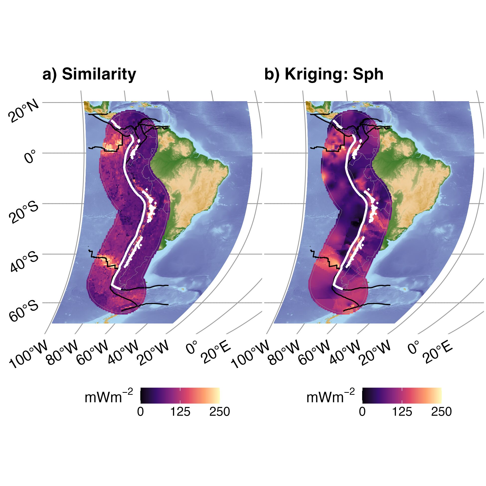
Figure B.7: Similarity (a) and Kriging (b) interpolations for Andes. Refer to the main text for explanation of panels and colors.

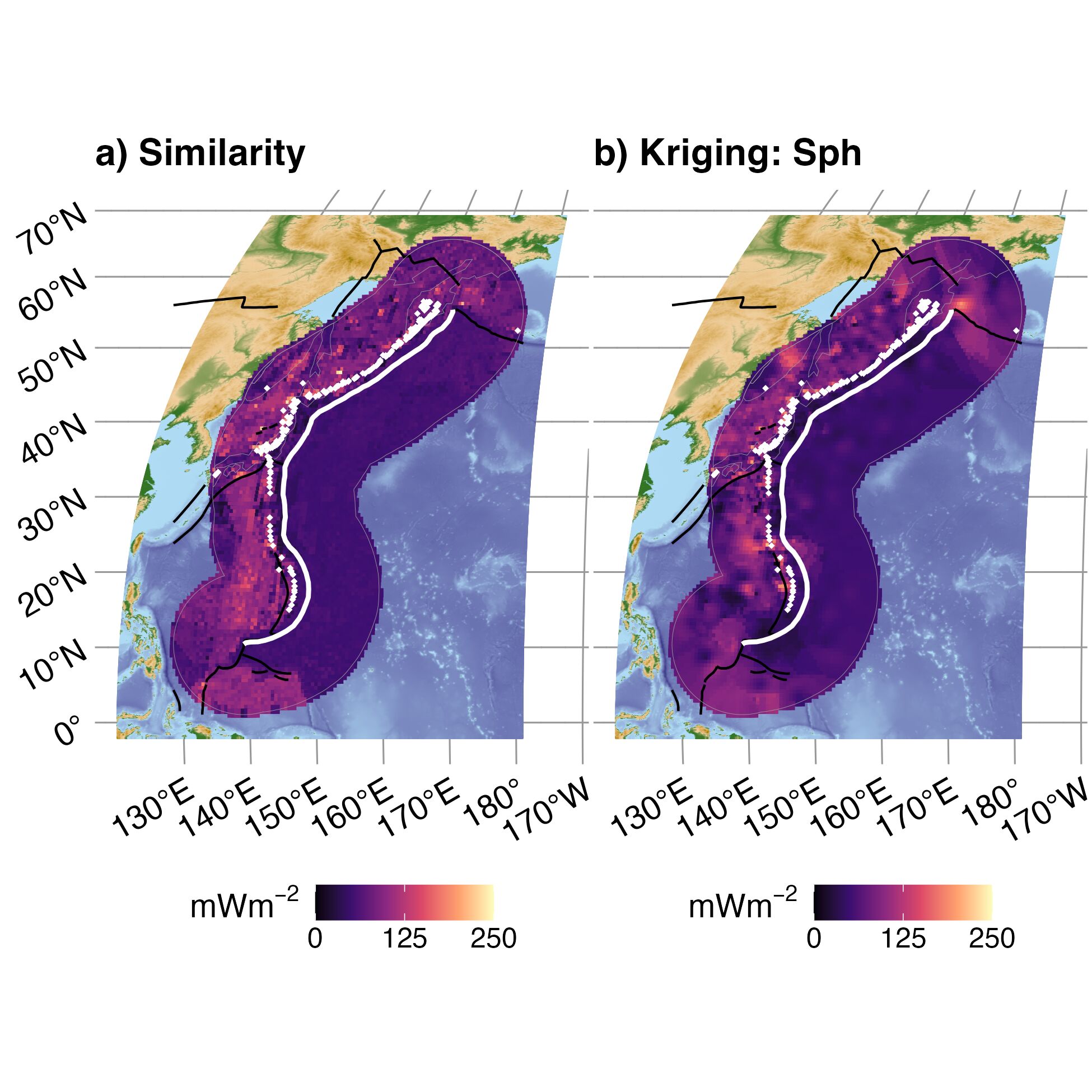
Figure B.8: Similarity (a) and Kriging (b) interpolations for Kamchatka Marianas. Refer to the main text for explanation of panels and colors.

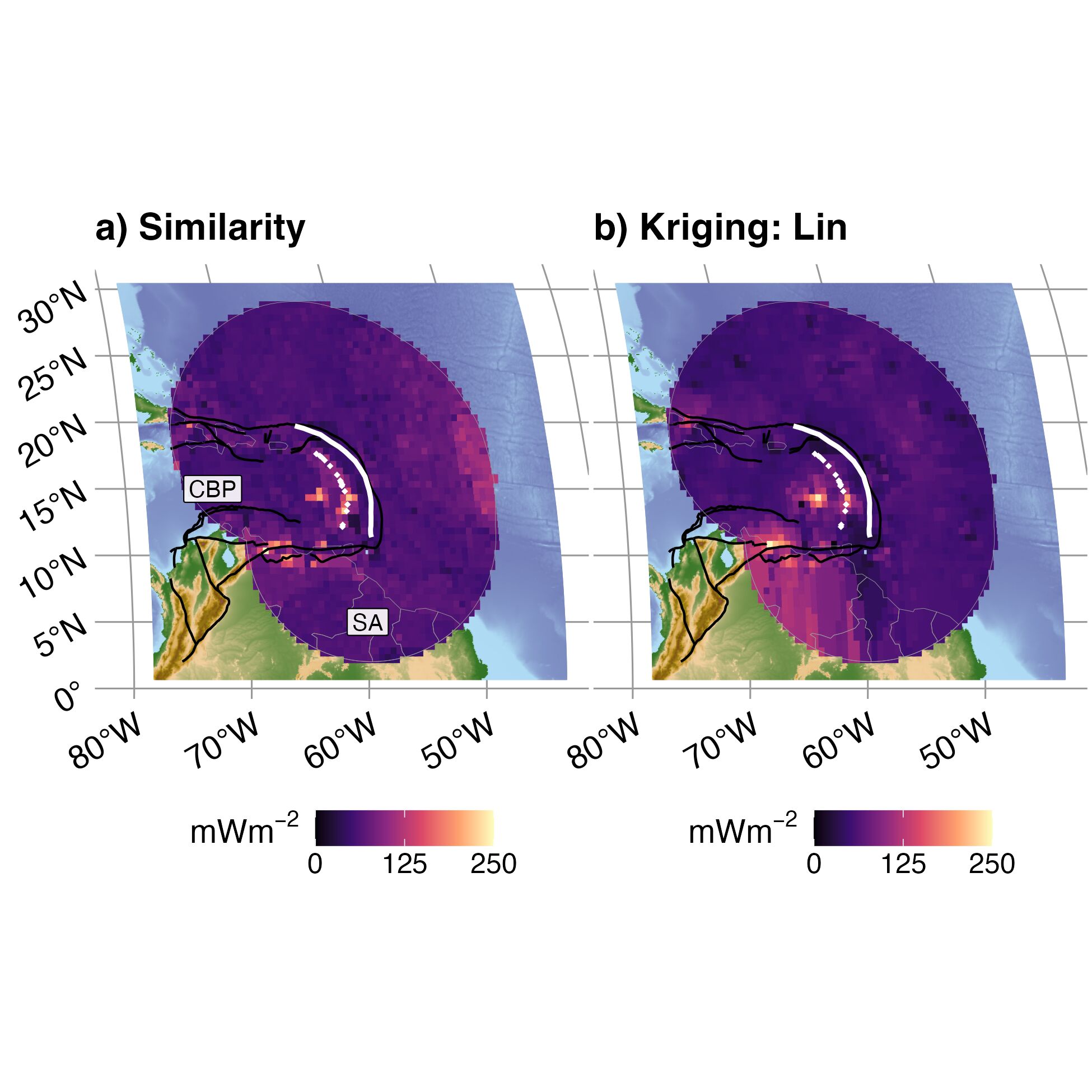
Figure B.9: Similarity (a) and Kriging (b) interpolations for Lesser Antilles. Refer to the main text for explanation of panels and colors.

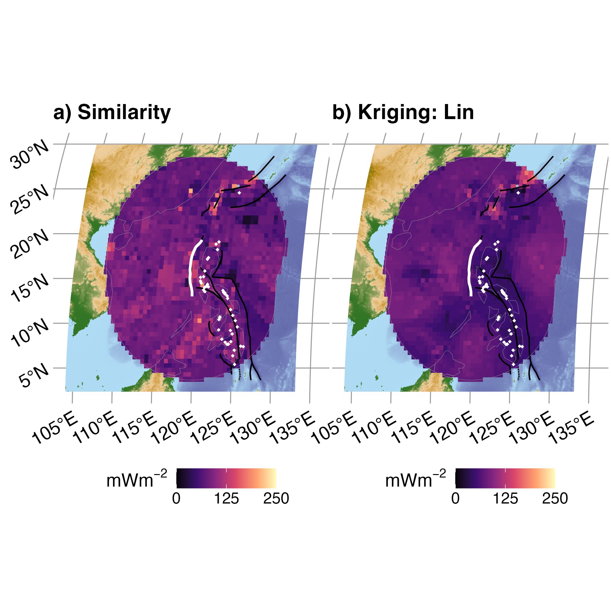
Figure B.10: Similarity (a) and Kriging (b) interpolations for N Philippines. Refer to the main text for explanation of panels and colors.

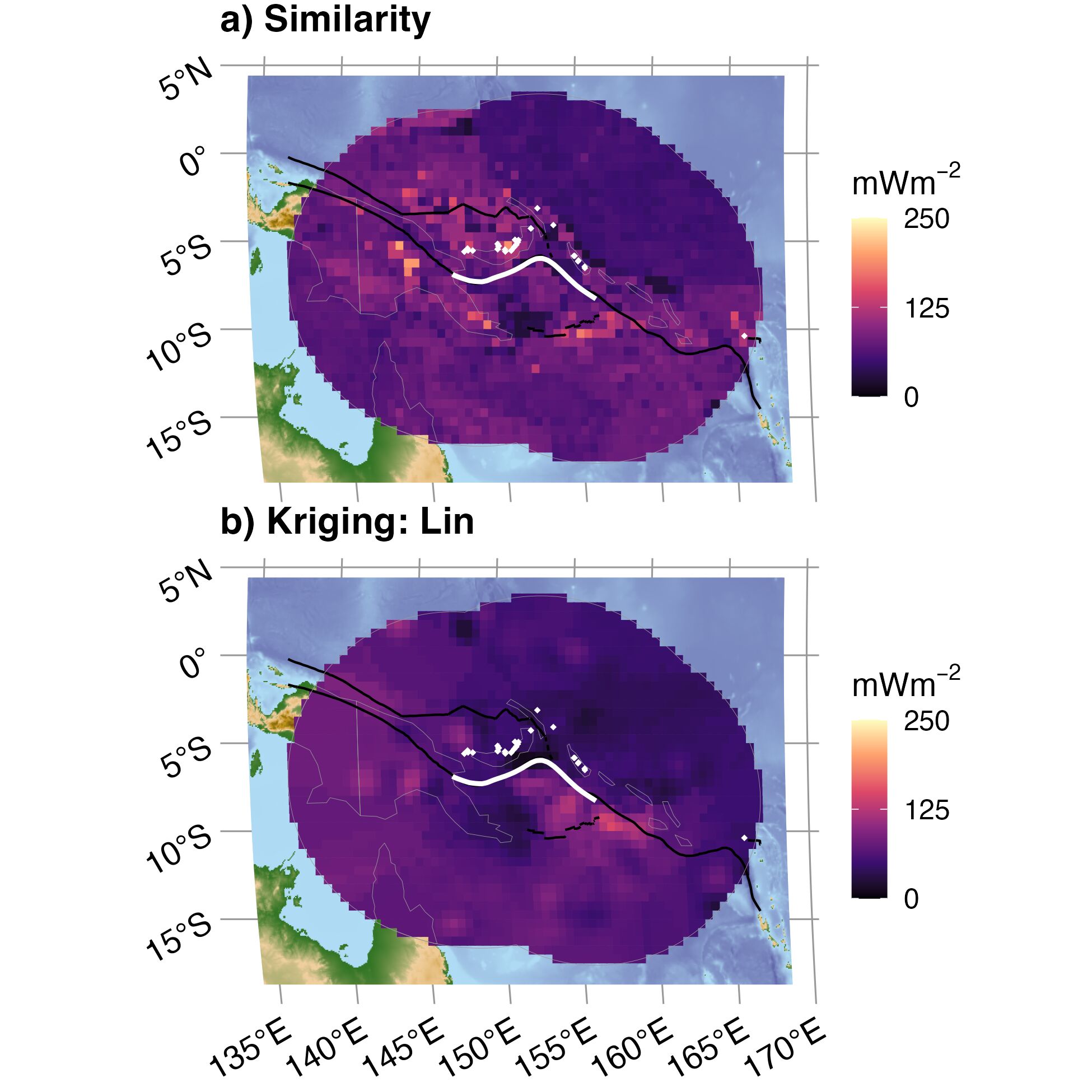
Figure B.11: Similarity (a) and Kriging (b) interpolations for New Britain Solomon. Refer to the main text for explanation of panels and colors.

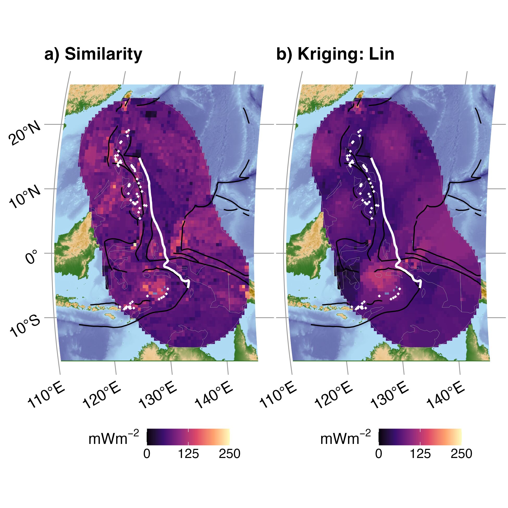
Figure B.12: Similarity (a) and Kriging (b) interpolations for S Philippines. Refer to the main text for explanation of panels and colors.

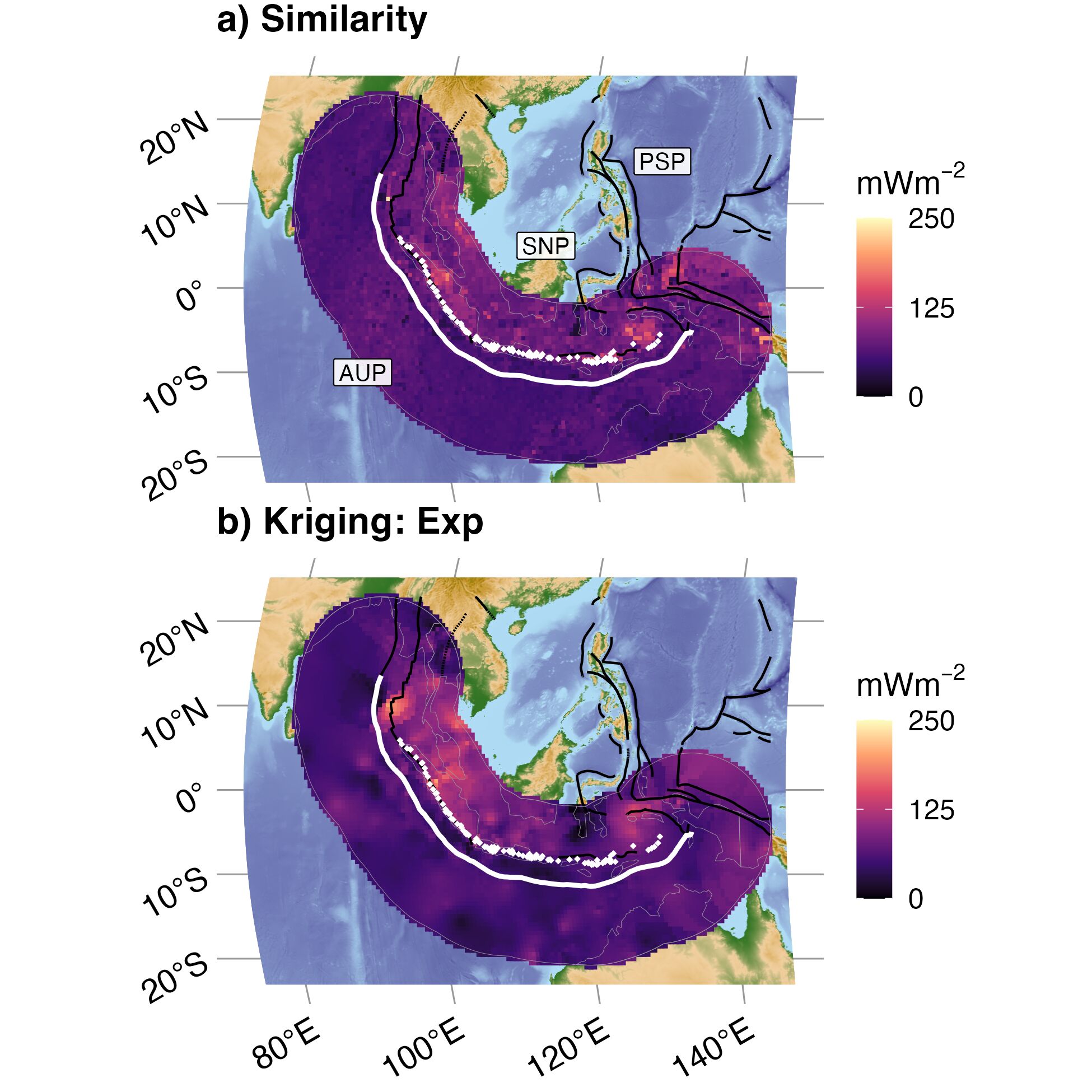
Figure B.13: Similarity (a) and Kriging (b) interpolations for Sumatra Banda Sea. Refer to the main text for explanation of panels and colors.

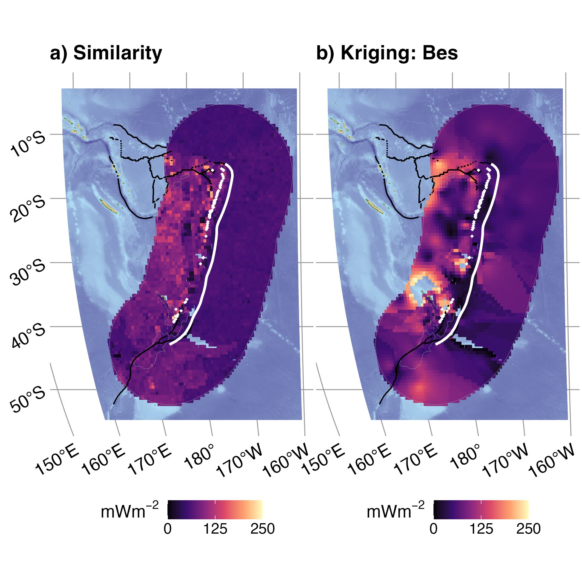
Figure B.14: Similarity (a) and Kriging (b) interpolations for Tonga New Zealand. Refer to the main text for explanation of panels and colors.

B.5 Upper-plate Surface Heat Flow

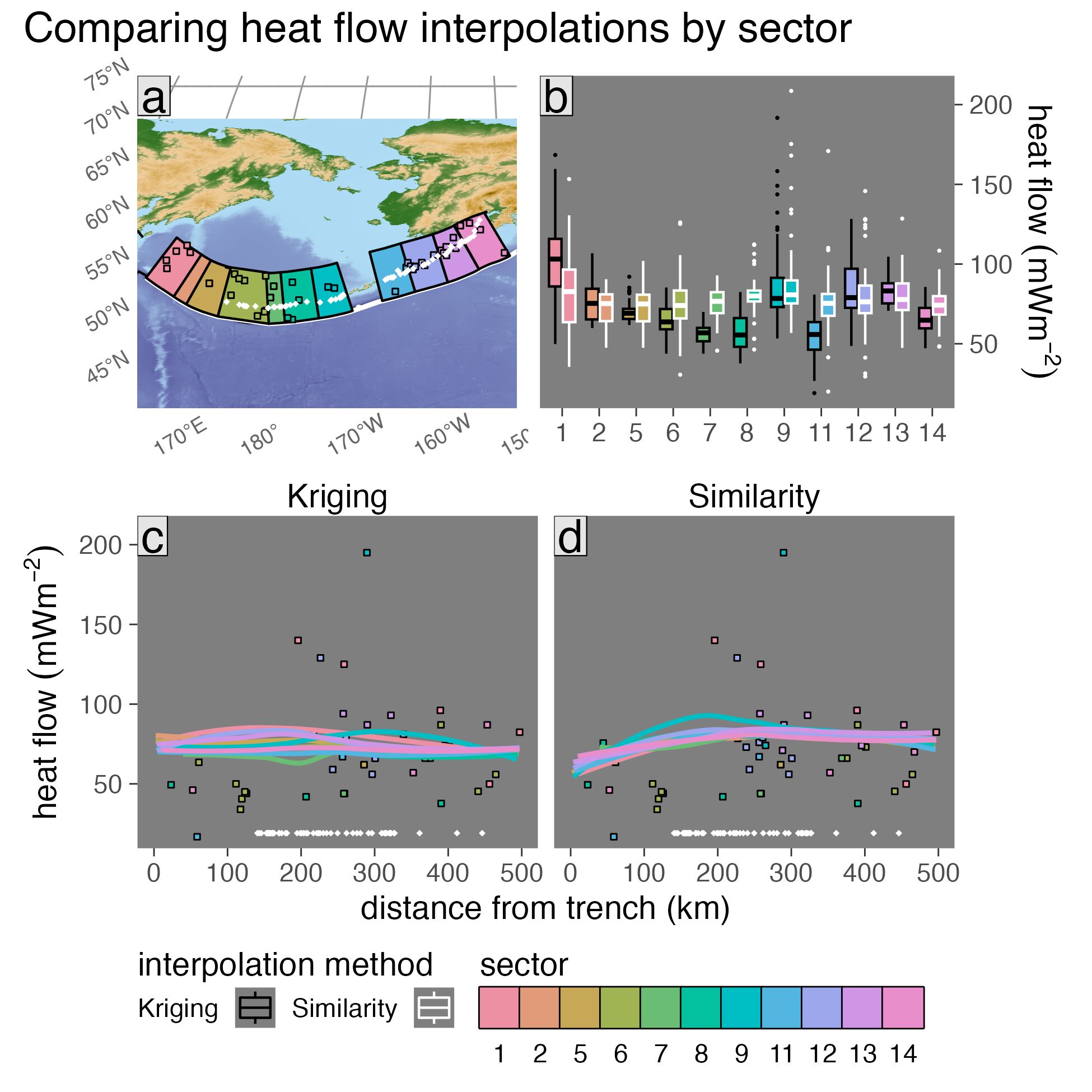
Figure B.15: Surface heat flow profiles for Alaska Aleutians upper-plate sectors. Refer to the main text for explanation of panels and colors.

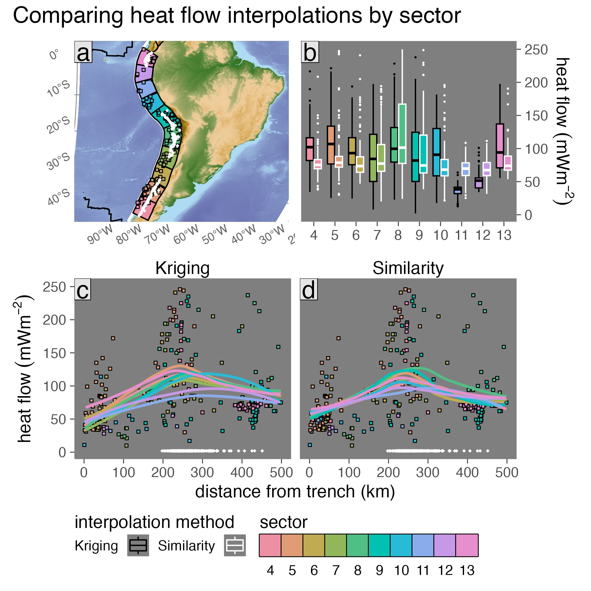
Figure B.16: Surface heat flow profiles for Andes upper-plate sectors. Refer to the main text for explanation of panels and colors.

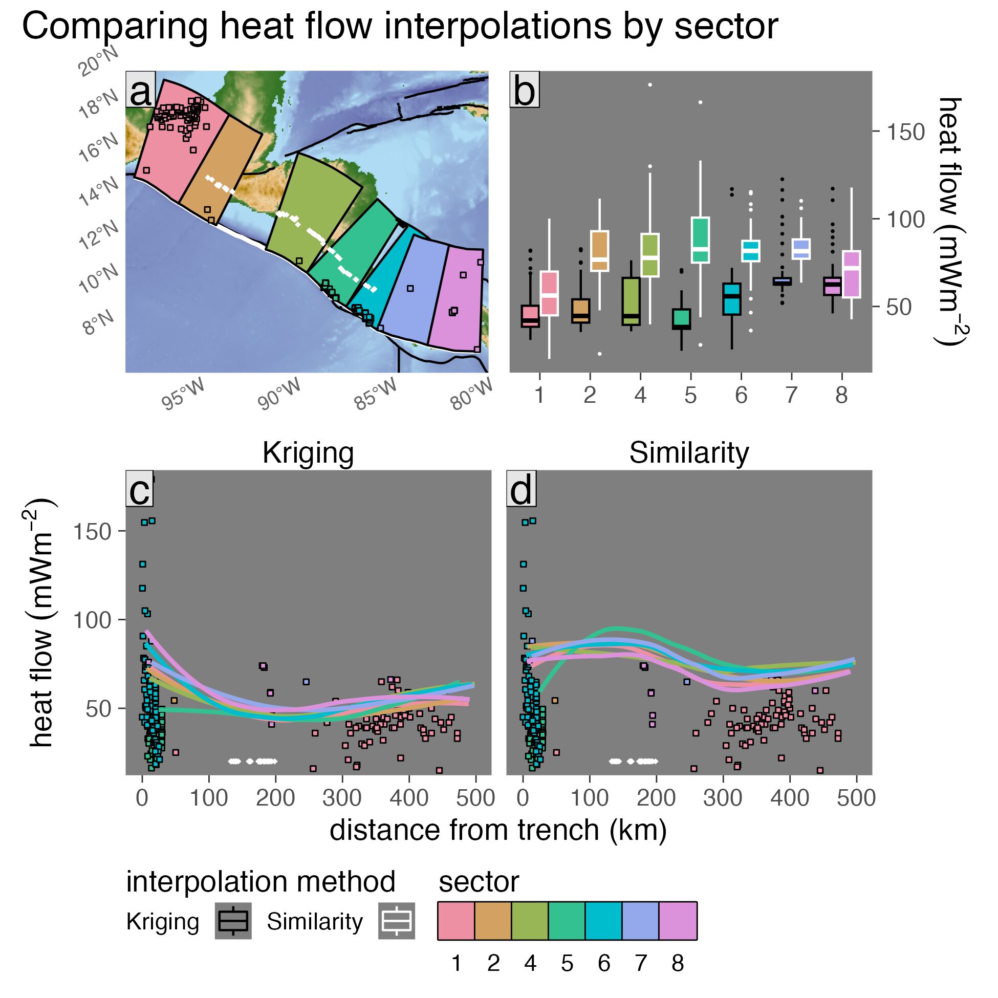
Figure B.17: Surface heat flow profiles for Central America upper-plate sectors. Refer to the main text for explanation of panels and colors.

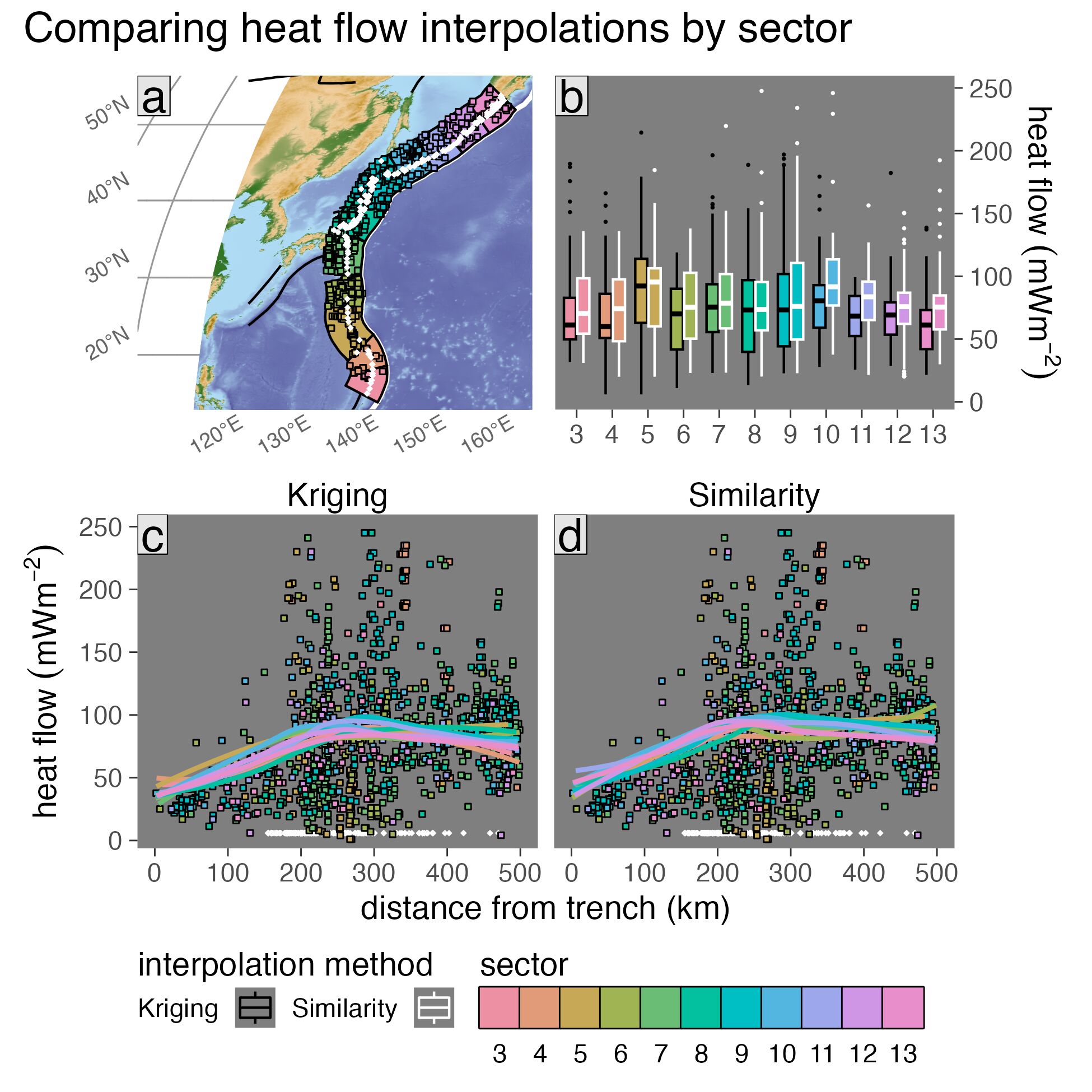
Figure B.18: Surface heat flow profiles for Kamchatka Marianas upper-plate sectors. Refer to the main text for explanation of panels and colors.

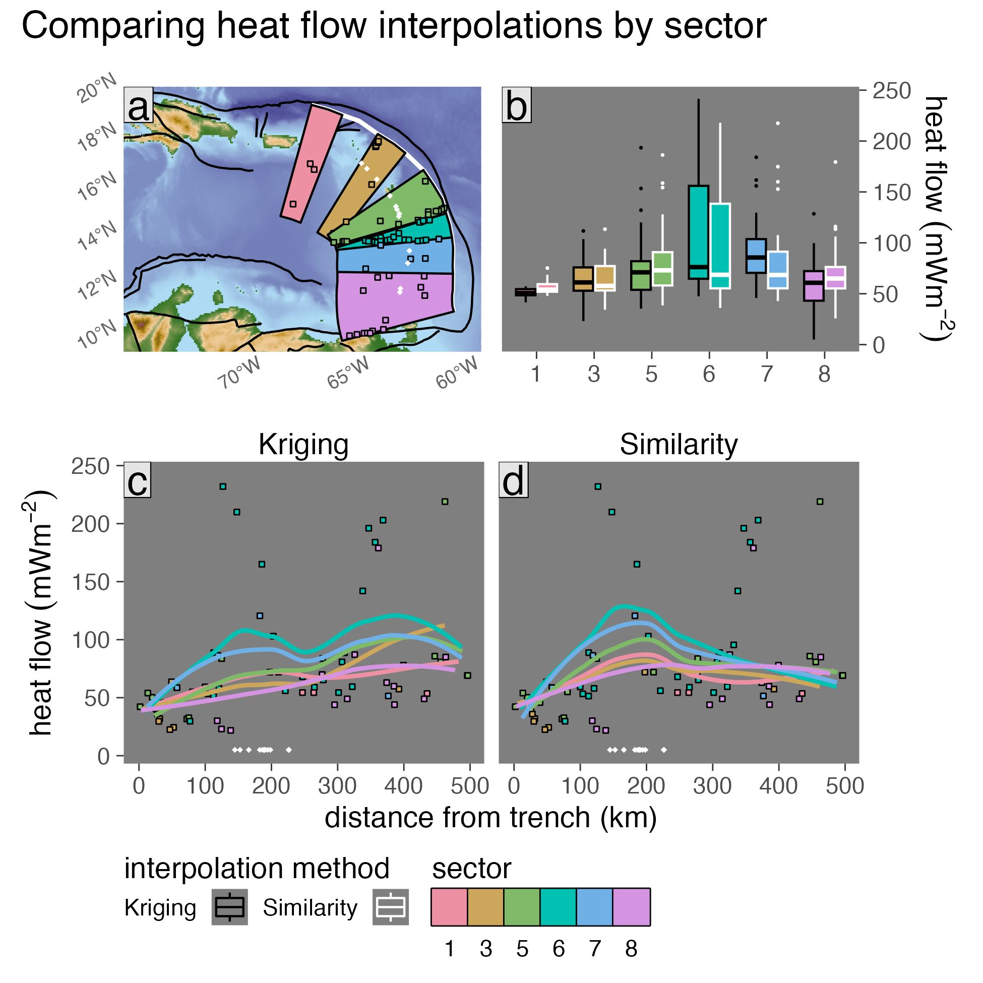
Figure B.19: Surface heat flow profiles for Lesser Antilles upper-plate sectors. Refer to the main text for explanation of panels and colors.

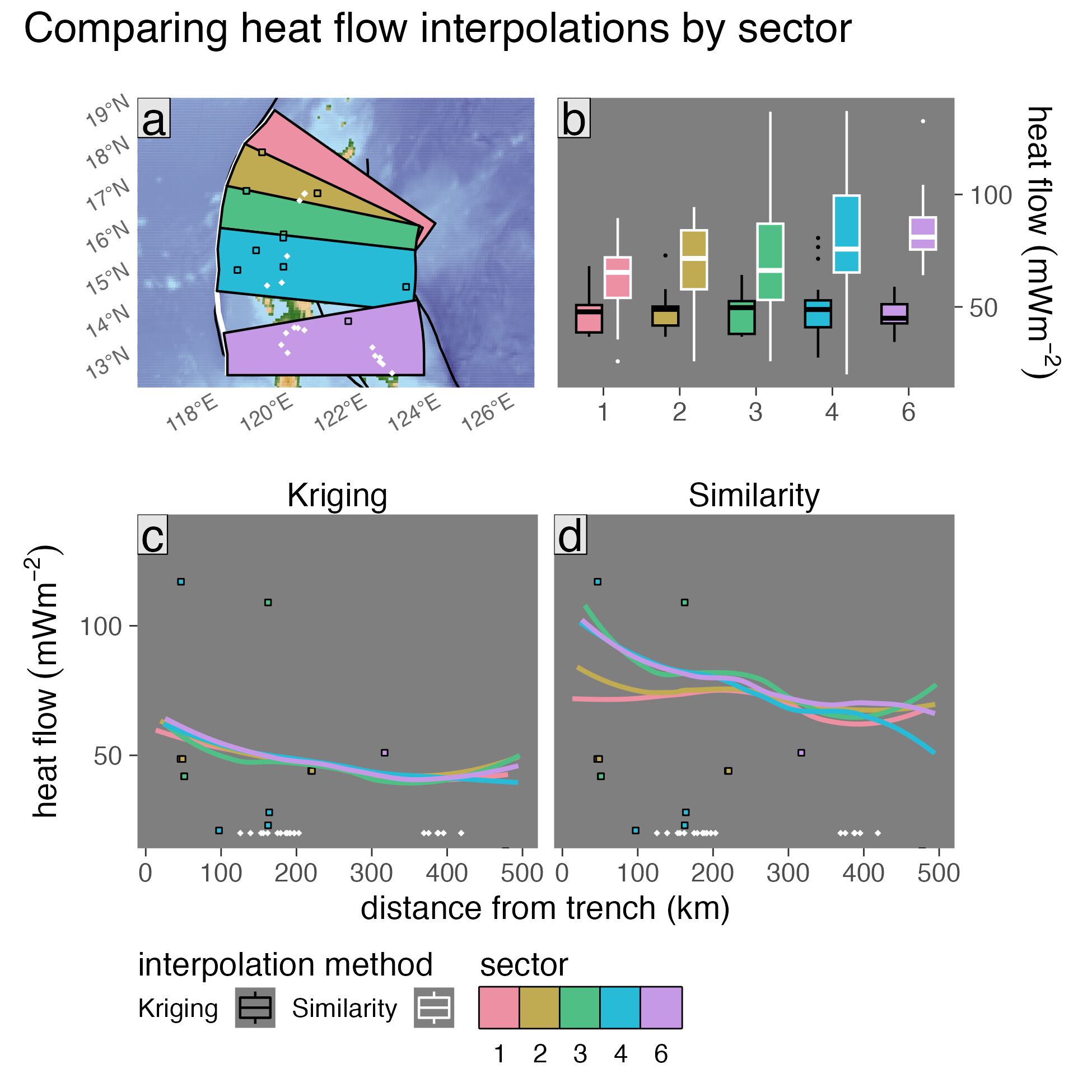
Figure B.20: Surface heat flow profiles for N Philippines upper-plate sectors. Refer to the main text for explanation of panels and colors.

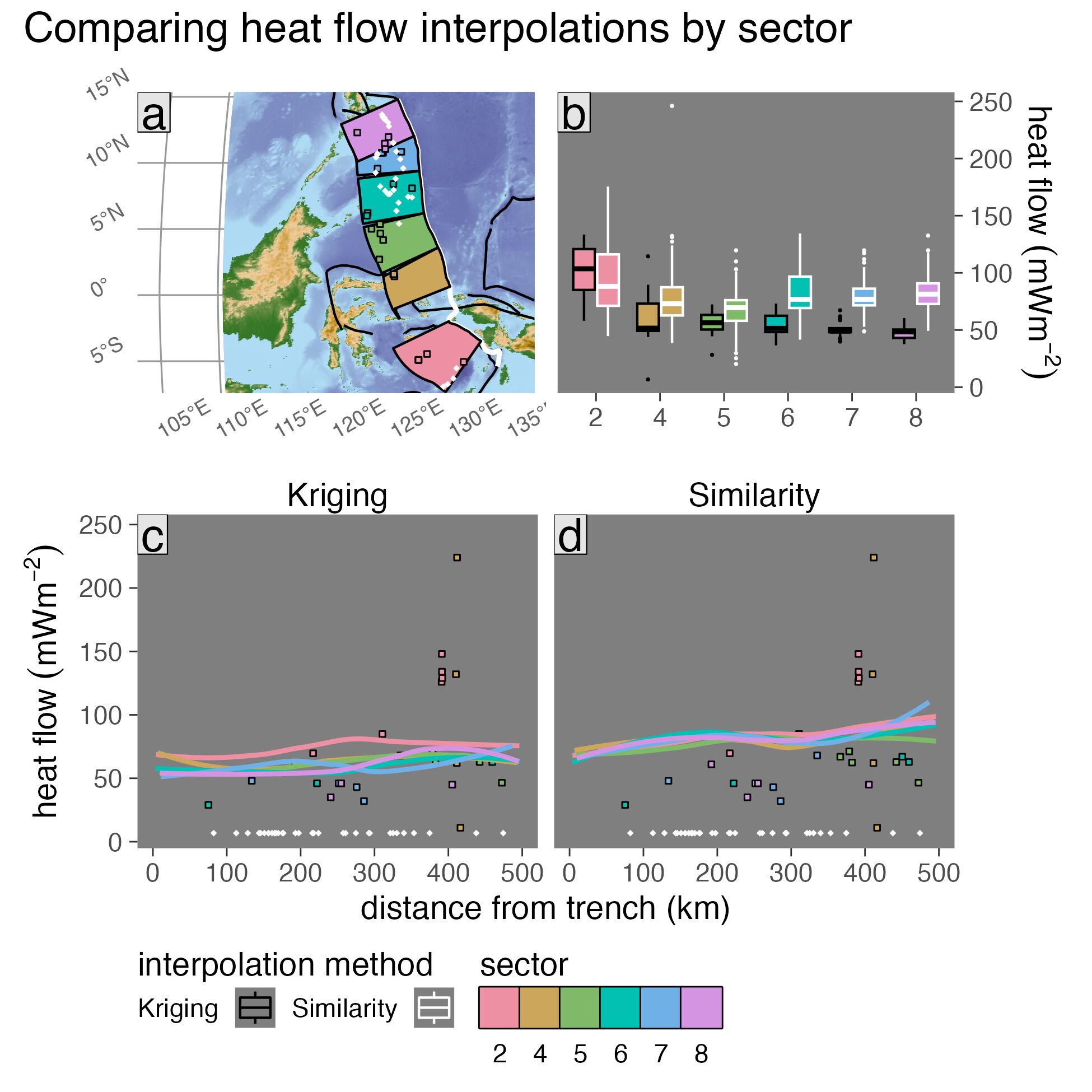
Figure B.21: Surface heat flow profiles for S Philippines upper-plate sectors. Refer to the main text for explanation of panels and colors.

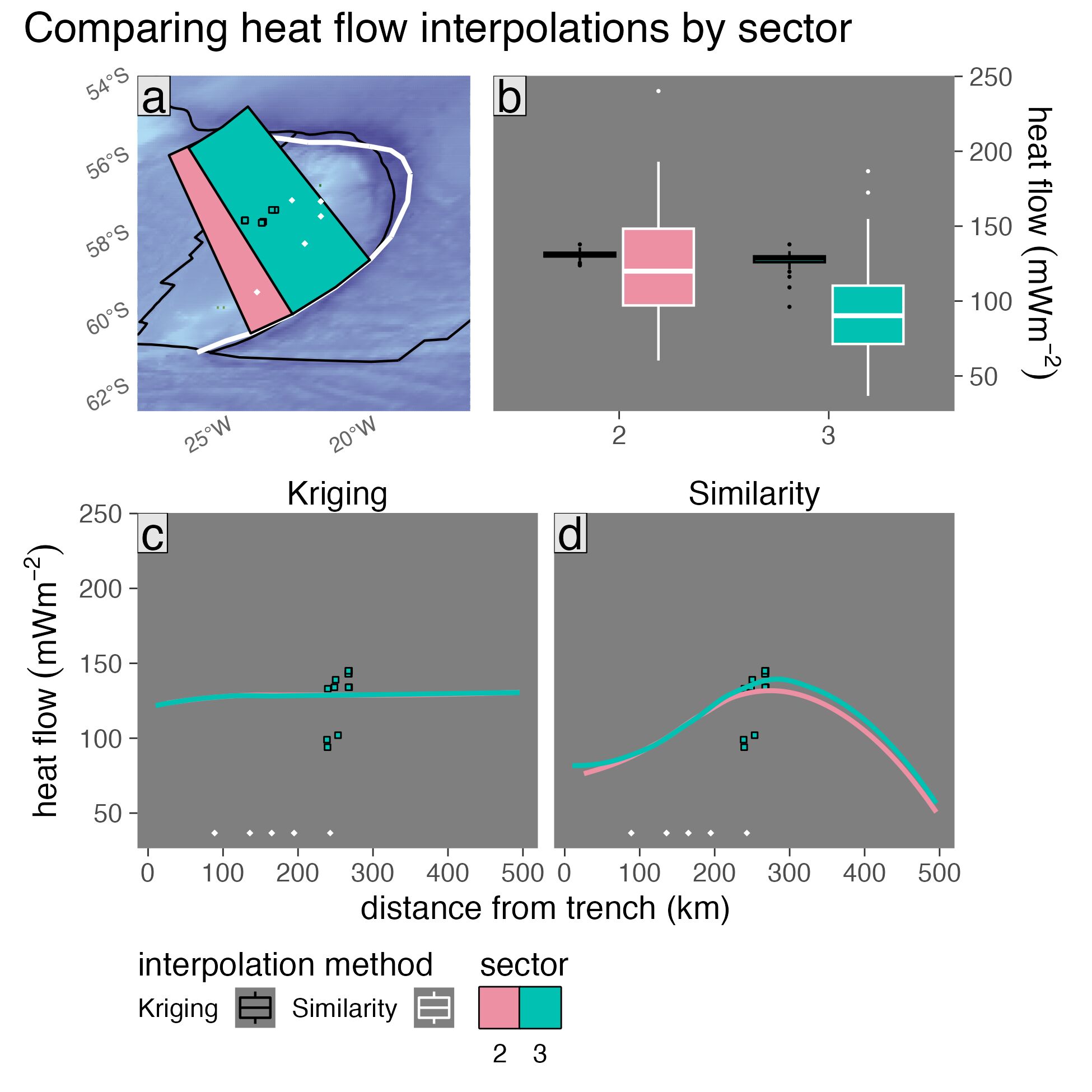
Figure B.22: Surface heat flow profiles for Scotia upper-plate sectors. Refer to the main text for explanation of panels and colors.

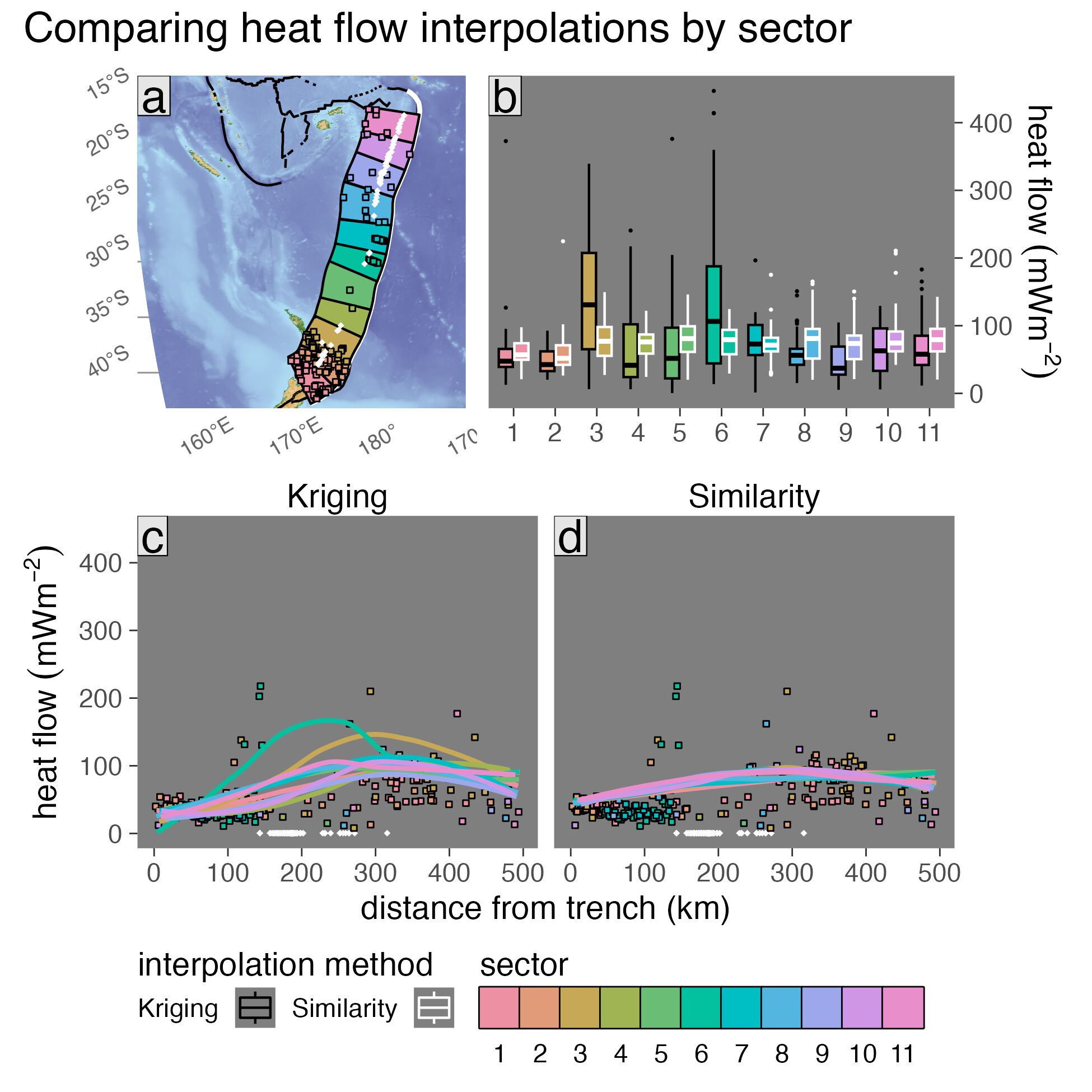
Figure B.23: Surface heat flow profiles for Tonga New Zealand upper-plate sectors. Refer to the main text for explanation of panels and colors.

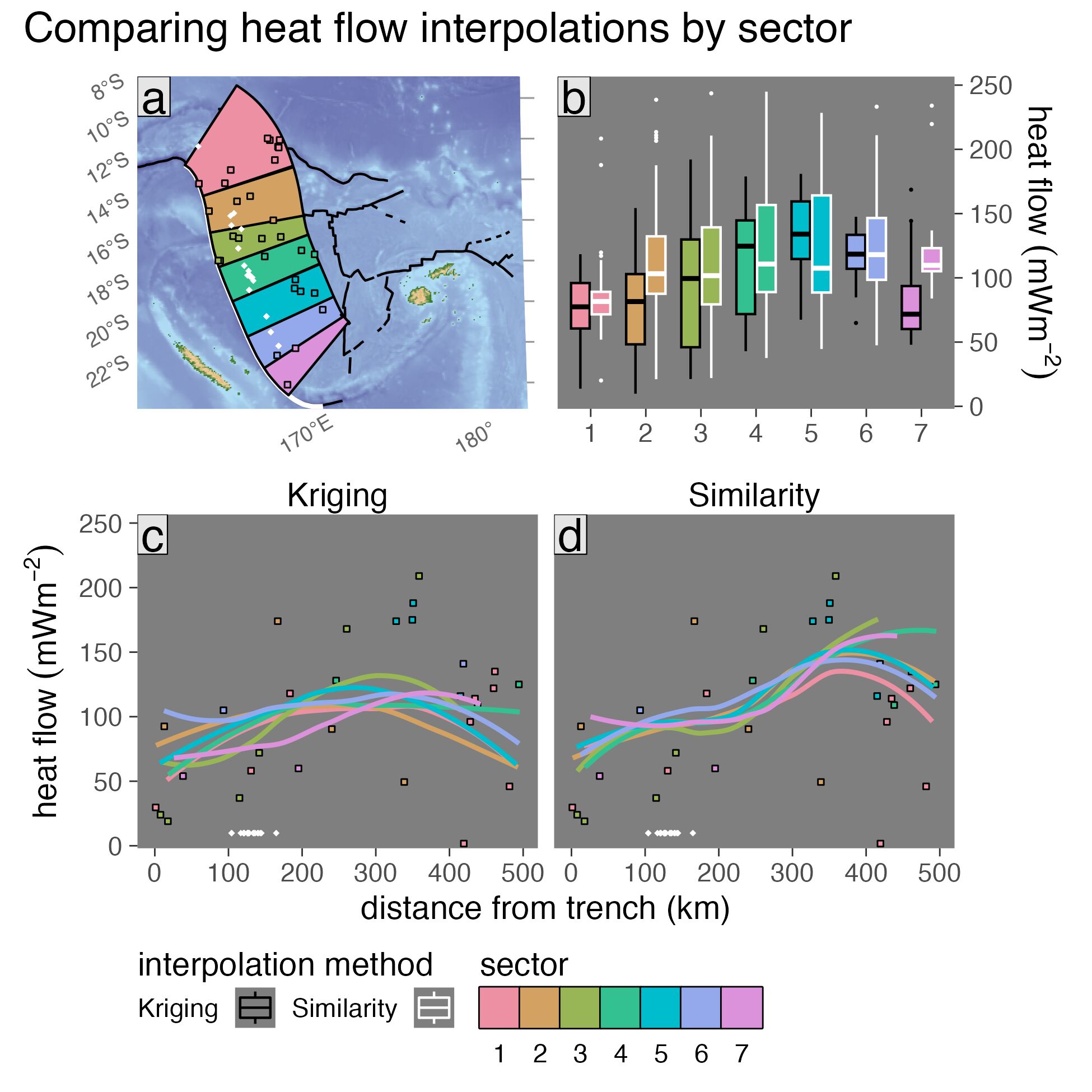
Figure B.24: Surface heat flow profiles for Vanuatu upper-plate sectors. Refer to the main text for explanation of panels and colors.

Table B.5: Summary of upper-plate surface heat flow

		ThermoGlobe			Similarity			Kriging
Segment	Sector	n	Median	IQR	n	Median	IQR	Median	IQR
Alaska Aleutians	1	5	96.1	42.6	80	82.7	33.0	103.0	34.0
Alaska Aleutians	2	1	62.0	0.0	69	75.2	16.8	74.6	18.4
Alaska Aleutians	5	1	62.0	0.0	68	75.0	16.7	68.7	7.7
Alaska Aleutians	6	13	50.0	22.2	115	74.0	17.5	64.6	13.7
Alaska Aleutians	7	2	55.0	11.1	35	76.6	13.2	53.0	15.9
Alaska Aleutians	8	4	45.6	15.1	79	79.9	6.8	56.1	19.3
Alaska Aleutians	9	2	134.6	60.5	74	80.7	14.4	83.5	32.7
Alaska Aleutians	11	2	41.9	25.1	84	75.3	13.7	53.0	16.3
Alaska Aleutians	12	8	74.5	15.2	86	76.3	17.3	78.4	36.1
Alaska Aleutians	13	6	84.0	15.8	72	77.8	16.7	83.3	15.2
Alaska Aleutians	14	4	63.5	20.0	86	74.2	11.5	62.2	13.2
Andes	4	14	74.5	89.5	127	75.3	13.8	104.0	31.5
Andes	5	68	69.0	59.8	114	78.7	16.1	114.3	41.2
Andes	6	39	61.0	40.5	122	73.6	23.4	99.7	31.2
Andes	7	23	81.0	112.0	120	77.3	40.3	94.0	67.7
Andes	8	30	94.0	69.2	141	101.4	89.6	101.4	46.0
Andes	9	45	61.0	57.0	130	74.6	56.3	89.3	58.2
Andes	10	11	45.0	19.5	94	68.2	24.7	86.9	48.1
Andes	11	4	41.9	8.3	88	69.8	19.2	39.6	6.5
Andes	12	4	36.0	8.2	91	67.4	19.8	51.8	11.1
Andes	13	36	71.0	7.0	88	74.0	21.2	101.4	59.9
Central America	1	72	42.0	13.0	64	56.2	24.9	40.8	15.5
Central America	2	2	50.2	4.1	41	76.7	22.6	35.7	21.9
Central America	4	1	37.7	0.0	59	77.7	24.2	45.6	18.1
Central America	5	41	34.7	6.6	39	82.6	25.7	40.9	12.3
Central America	6	94	50.9	20.1	39	81.7	11.6	59.3	21.3
Central America	7	2	76.4	11.5	48	81.5	11.1	66.3	4.3
Central America	8	10	63.0	15.1	44	71.8	26.4	63.6	16.3
Kamchatka Marianas	3	25	186.0	112.0	81	70.4	44.1	59.1	48.6
Kamchatka Marianas	4	43	64.5	150.8	78	74.2	49.2	60.6	37.7
Kamchatka Marianas	5	79	54.0	63.5	123	95.4	46.2	87.8	50.2
Kamchatka Marianas	6	116	69.6	64.5	86	75.3	52.5	67.4	51.4
Kamchatka Marianas	7	301	75.0	50.0	113	78.6	43.3	76.3	42.1
Kamchatka Marianas	8	126	81.8	55.0	118	73.6	38.4	69.8	55.0
Kamchatka Marianas	9	172	89.0	82.8	153	76.0	61.0	72.4	57.2
Kamchatka Marianas	10	59	83.7	30.8	98	91.7	36.7	80.7	33.7
Kamchatka Marianas	11	27	80.0	39.8	94	83.7	30.6	68.7	32.4
Kamchatka Marianas	12	48	78.2	41.2	117	75.8	24.8	69.7	25.7
Kamchatka Marianas	13	55	68.0	36.5	108	75.5	27.1	61.6	31.1
Kyushu Ryukyu	1	74	69.5	41.8	52	75.8	40.3	78.9	29.8
Kyushu Ryukyu	2	25	80.0	40.0	43	77.6	13.1	76.6	16.0
Kyushu Ryukyu	3	6	67.5	18.2	61	86.2	17.8	74.9	37.3
Kyushu Ryukyu	4	28	77.5	26.2	43	84.9	24.6	93.0	49.0
Kyushu Ryukyu	5	103	88.0	77.0	48	72.4	27.2	74.3	39.3
Kyushu Ryukyu	6	25	126.0	94.0	39	80.4	19.0	81.7	70.0
Kyushu Ryukyu	7	42	60.0	70.2	33	76.3	16.7	64.2	53.1
Kyushu Ryukyu	8	36	43.4	30.8	23	62.1	37.6	49.5	35.5
Lesser Antilles	1	3	54.4	0.4	23	54.0	7.5	49.9	4.8
Lesser Antilles	3	10	38.1	31.9	20	57.7	24.0	59.4	26.7
Lesser Antilles	5	15	55.0	36.2	29	73.0	32.7	71.4	36.2
Lesser Antilles	6	24	74.4	89.3	17	68.6	83.1	81.1	103.9
Lesser Antilles	7	6	78.2	26.8	29	68.4	36.0	84.0	34.3
Lesser Antilles	8	14	54.5	32.0	46	64.9	20.3	59.5	21.7
N Philippines	1	2	46.3	2.3	30	65.3	18.0	45.4	11.6
N Philippines	2	3	44.0	3.3	20	71.6	26.2	45.9	11.7
N Philippines	3	2	75.4	33.5	17	66.2	33.9	46.8	13.2
N Philippines	4	5	23.0	7.0	33	75.7	34.2	44.5	14.1
N Philippines	6	1	51.0	0.0	30	81.1	14.3	45.3	15.2
New Britain Solomon	3	1	37.7	0.0	26	83.2	24.9	38.9	13.3
New Britain Solomon	4	1	2.9	0.0	16	95.2	46.1	24.3	13.4
New Britain Solomon	5	3	36.8	12.1	64	57.9	29.5	43.1	9.6
New Britain Solomon	6	3	35.2	10.6	38	52.5	10.5	31.4	9.1
New Britain Solomon	8	1	58.2	0.0	19	56.6	27.8	45.7	5.4
S Philippines	2	6	127.5	37.6	83	88.2	45.0	102.8	19.2
S Philippines	4	4	97.0	105.8	62	73.0	24.7	49.0	11.9
S Philippines	5	5	62.8	4.6	68	69.6	18.0	56.1	12.6
S Philippines	6	3	62.8	19.0	72	76.8	27.4	48.6	24.8
S Philippines	7	5	46.0	5.0	46	76.9	14.6	46.7	5.5
S Philippines	8	4	45.5	7.2	65	81.4	18.0	44.4	4.8
Scotia	2	3	143.0	5.5	28	120.0	51.2	127.2	11.1
Scotia	3	9	134.0	37.0	54	90.2	38.9	127.1	8.9
Sumatra Banda Sea	1	339	21.0	10.8	69	74.4	15.2	86.4	123.3
Sumatra Banda Sea	3	23	80.0	24.2	59	75.4	22.6	70.2	23.7
Sumatra Banda Sea	4	208	113.0	46.2	112	85.2	32.1	90.5	42.6
Sumatra Banda Sea	5	192	123.0	32.5	95	85.4	36.9	100.4	58.9
Sumatra Banda Sea	6	40	103.0	13.0	73	72.9	50.0	67.2	62.1
Sumatra Banda Sea	7	86	70.5	31.5	72	71.7	24.7	71.7	30.0
Sumatra Banda Sea	8	40	78.0	18.5	64	66.7	18.0	56.2	26.7
Sumatra Banda Sea	9	30	77.5	25.2	83	68.8	28.8	42.5	39.1
Sumatra Banda Sea	10	5	75.0	51.2	91	70.7	24.7	53.8	18.4
Sumatra Banda Sea	11	1	71.2	0.0	67	72.3	12.4	62.4	7.5
Sumatra Banda Sea	12	0			85	80.0	19.0	69.3	20.5
Tonga New Zealand	1	75	47.0	39.0	44	56.9	24.3	47.9	21.1
Tonga New Zealand	2	44	39.5	20.8	34	49.7	29.0	42.6	18.5
Tonga New Zealand	3	30	64.0	36.0	64	73.6	38.2	95.3	90.0
Tonga New Zealand	4	1	24.3	0.0	48	76.0	28.2	49.8	60.8
Tonga New Zealand	5	1	15.1	0.0	68	80.7	37.4	40.5	51.2
Tonga New Zealand	6	29	31.2	15.0	48	79.7	35.6	127.9	120.0
Tonga New Zealand	7	35	28.5	7.1	53	71.9	24.0	47.4	32.0
Tonga New Zealand	8	7	49.0	49.2	64	81.0	43.8	58.0	24.1
Tonga New Zealand	9	4	31.1	23.2	58	73.8	34.8	53.1	46.2
Tonga New Zealand	10	4	59.7	47.0	48	74.3	29.3	71.0	48.9
Tonga New Zealand	11	5	31.8	19.7	52	79.3	33.4	53.8	41.1
Vanuatu	1	9	96.0	72.0	68	81.6	17.5	84.5	37.5
Vanuatu	2	4	91.4	32.7	44	103.0	51.3	79.8	49.8
Vanuatu	3	6	54.5	116.8	27	101.7	60.0	96.9	85.0
Vanuatu	4	3	125.0	9.5	34	110.8	67.7	119.4	87.2
Vanuatu	5	4	174.5	18.8	36	107.5	75.6	133.6	41.7
Vanuatu	6	2	123.0	18.0	30	118.1	48.1	110.0	29.8
Vanuatu	7	2	57.0	2.9	20	109.8	18.0	71.9	25.3
note: Similarity and Kriging prediction counts are the same. Surface heat flow units are mW/m\(^2\).

C Computing Rates and Distributions of Rock Recovery in Subduction Zones

C.1 Gaussian Mixture Models

Let the traced markers represent a \(d\)-dimensional array of \(n\) random independent variables \(x_i \in \mathbb{R}^{n \times d}\). Assume markers \(x_i\) were drawn from \(k\) discrete probability distributions with parameters \(\Phi\). The probability distribution of markers \(x_i\) can be modeled with a mixture of \(k\) components: \[\begin{equation} p(x_i | \Phi) = \sum_{j=1}^k \pi_j p(x_i | \Theta_j) \tag{C.1} \end{equation}\] where \(p(x_i | \Theta_j)\) is the probability of \(x_i\) under the \(j^{th}\) mixture component and \(\pi_j\) is the mixture proportion representing the probability that \(x_i\) belongs to the \(j^{th}\) component \((\pi_j \geq 0; \sum_{j=1}^k \pi_j = 1)\).

Assuming \(\Theta_j\) describes a Gaussian probability distributions with mean \(\mu_j\) and covariance \(\Sigma_j\), Equation (C.1) becomes: \[\begin{equation} p(x_i | \Phi) = \sum_{j=1}^k \pi_j \mathcal{N}(x_i | \mu_j, \Sigma_j) \tag{C.2} \end{equation}\] where \[\begin{equation} \mathcal{N}(x_i | \mu_j, \Sigma_j) = \frac{exp\{ -\frac{1}{2}(x_i - \mu_j)(x_i - \mu_j)^T \Sigma_j^{-1}\}}{\sqrt{det(2 \pi \Sigma_j)}} \tag{C.3} \end{equation}\]

The parameters \(\mu_j\) and \(\Sigma_j\), representing the center and shape of each cluster, are estimated by maximizing the log of the likelihood function, \(L(x_i | \Phi) = \prod_{i=1}^n p(x_i | \Phi)\): \[\begin{equation} log~L(x_i | \Phi) = log \prod_{i=1}^n p(x_i | \Phi) = \sum_{i=1}^n log \left[ \sum_{j=1}^k \pi_j p(x_i | \Theta_j) \right] \tag{C.4} \end{equation}\]

Taking the derivative of Equation (C.4) with respect to each parameter, \(\pi\), \(\mu\), \(\Sigma\), setting the equation to zero, and solving for each parameter gives the maximum likelihood estimators: \[\begin{equation} \begin{aligned} N_j &= \sum_{i=1}^n \omega_{i} \\ \pi_j &= \frac{N_j}{n} \\ \mu_j &= \frac{1}{N_j} \sum_{i=1}^n \omega_{i} x_i \\ \Sigma_j &= \frac{1}{N_j} \sum_{i=1}^n \omega_{i} (x_i - \mu_j)(x_i - \mu_j)^T \end{aligned} \tag{C.5} \end{equation}\] where \(\omega_{i}\) (\(\omega_{i} \geq 0; \sum_{j=1}^k \omega_{i} = 1\)) are membership weights representing the probability of an observation \(x_i\) belonging to the \(j^{th}\) Gaussian and \(N_j\) represents the number of observations belonging to the \(j^{th}\) Gaussian. Please note that \(\omega_{i}\) is unknown for markers so the maximum likelihood estimator cannot be computed with Equation (C.5). The solution to this problem is the Expectation-Maximization algorithm, which is defined below.

General purpose functions in the R package Mclust (Scrucca et al., 2016) are used to fit Gaussian mixture models. “Fitting” refers to adjusting all \(k\) Gaussian parameters \(\mu_j\) and \(\Sigma_j\) until the data and Gaussian ellipsoids achieve maximum likelihood defined by Equation (C.4). After Banfield & Raftery (1993), covariance matrices \(\Sigma\) in Mclust are parameterized to be flexible in their shape, volume, and orientation (Scrucca et al., 2016): \[\begin{equation} \Sigma_j = \lambda_j D_j A_j D_j^T \tag{C.6} \end{equation}\] where \(D_j\) is the orthogonal eigenvector matrix, \(A_j\) and \(\lambda_j\) are diagonal matrices of values proportional to the eigenvalues. This implementation allows fixing one, two, or three geometric elements of the covariance matrices. That is, the volume \(\lambda_j\), shape \(A_j\), and orientation \(D_j\) of Gaussian clusters can change or be fixed among all \(k\) clusters (e.g., Celeux & Govaert, 1995; Fraley & Raftery, 2002). Fourteen parameterizations of Equation (C.6) are tried, representing different geometric combinations of the covariance matrices \(\Sigma\) (see Scrucca et al., 2016) and the Bayesian information criterion is computed (Schwarz, 1978). The parameterization for Equation (C.6) is chosen by Bayesian information criterion.

C.2 Expectation-Maximization

The Expectation-Maximization algorithm estimates Gaussian mixture model parameters by initializing \(k\) Gaussians with parameters \((\pi_j, \mu_j, \Sigma_j)\), then iteratively computing membership weights with Equation (C.7) and updating Gaussian parameters with Equation (C.5) until reaching a convergence threshold (Dempster et al., 1977).

The expectation (E-)step involves a “latent” multinomial variable \(z_{i} \in \{1, 2, \dots, k\}\) representing the unknown classifications of \(x_i\) with a joint distribution \(p(x_i,z_{i}) = p(x_i | z_{i})p(z_{j})\). Membership weights \(\omega_{i}\) are equivalent to the conditional probability \(p(z_{i} | x_i)\), which represents the probability of observation \(x_i\) belonging to the \(j^{th}\) Gaussian. Given initial guesses for Gaussian parameters \(\pi_j\), \(\mu_j\), \(\Sigma_j\), membership weights are computed using Bayes Theorem (E-step): \[\begin{equation} p(z_{i} | x_i) = \frac{p(x_i | z_{i})p(z_{j})}{p(x_i)} = \frac{\pi_j \mathcal{N}(\mu_j, \Sigma_j)}{\sum_{j=1}^k \pi_j \mathcal{N}(\mu_j, \Sigma_j)} = \omega_{i} \tag{C.7} \end{equation}\] and Gaussian estimates are updated during the maximization (M-)step by applying \(\omega_{i}\) to Equation (C.5). This step gives markers \(x_i\) class labels \(z_i \in \{1, \dots, k\}\) representing assignment to one of \(k\) clusters (Figure 4.2).

C.3 Marker Classification Results

Below are the classification results for all 64 numerical experiments presented in the main text (Table C.1).

Table C.1: Subduction zone parameters and marker classification summary

Initial Boundary Conditions					Marker Classification Summary
model	\(\Phi\)	\(Z_{UP}\)	age	\(\vec{v}\)	recovered	rec. rate	P mode1	P mode2	T mode1	T mode2	grad mode1	grad mode2
	km	km	Ma	km/Ma		%	GPa	GPa	˚C	˚C	˚C/km	˚C/km
cda46	13.0	46	32.6	40	1481±26	7.8±0.14	1.12±0.00	2.46±0.04	336±2	570±176	8.2±0.02	9.5±0.08
cda62	13.0	62	32.6	40	1349±22	7.1±0.12	1.12±0.00	2.22±0.22	333±0	529±2	8.3±0.02	8.3±0.02
cda78	13.0	78	32.6	40	1862±28	9.9±0.14	1.39±0.00	2.39±0.02	352±2	476±2	5.9±0.02	9±2.12
cda94	13.0	94	32.6	40	1932±24	10.2±0.14	1.24±0.00	2.64±0.00	341±0	499±2	5.6±0.00	7.8±0.02
cdb46	21.5	46	32.6	66	1815±28	9.6±0.14	1.04±0.00	2.36±0.74	334±2	668±96	8.3±0.04	8.3±0.04
cdb62	21.5	62	32.6	66	1408±28	7.5±0.14	1±0.00	2.16±0.00	281±2	535±24	7.8±0.04	10±0.06
cdb78	21.5	78	32.6	66	1882±30	10±0.16	0.92±0.00	2.49±0.08	264±2	542±8	8.1±0.02	8.1±0.02
cdb94	21.5	94	32.6	66	2359±36	12.5±0.20	1.13±0.00	2.63±0.02	291±0	460±2	7.5±0.02	8±1.34
cdc46	26.1	46	32.6	80	1736±38	9.2±0.20	1.02±0.00	1.27±0.68	320±2	451±120	8.7±0.30	9±1.04
cdc62	26.1	62	32.6	80	1292±30	6.8±0.16	0.99±0.00	2.01±0.00	264±2	531±2	6.7±0.02	8.7±0.26
cdc78	26.1	78	32.6	80	1807±22	9.6±0.12	0.95±0.12	2.87±0.16	283±2	512±12	7.8±0.02	8.1±2.00
cdc94	26.1	94	32.6	80	2153±26	11.4±0.14	1.14±0.00	2.99±0.14	274±0	533±4	6.7±0.02	9.8±0.04
cdd46	32.6	46	32.6	100	1049±58	5.6±0.32	0.99±0.00	1.76±0.14	227±2	470±2	6±0.04	8.5±0.06
cdd62	32.6	62	32.6	100	1366±24	7.2±0.12	0.99±0.00	1.65±0.20	263±2	333±46	5.6±0.10	8.9±0.04
cdd78	32.6	78	32.6	100	1890±32	10±0.16	0.99±0.00	1.94±0.00	264±2	512±2	7.5±0.02	11.7±1.86
cdd94	32.6	94	32.6	100	2711±24	14.4±0.12	1.23±0.00	2.9±0.02	244±46	661±4	7.3±0.04	7.3±0.04
cde46	22.0	46	55.0	40	1614±42	8.5±0.22	1.11±0.00	2.95±0.88	316±2	698±92	6.7±0.02	8.1±1.08
cde62	22.0	62	55.0	40	1800±38	9.5±0.20	1.08±0.00	2.24±0.00	285±4	485±2	6.1±0.02	7.3±0.66
cde78	22.0	78	55.0	40	1870±24	9.9±0.12	1.36±0.00	2.52±0.00	315±2	496±2	5.8±0.08	7.5±0.02
cde94	22.0	94	55.0	40	1807±28	9.6±0.14	2.34±0.86	2.54±0.00	319±2	430±2	5±0.00	7.2±0.02
cdf46	36.3	46	55.0	66	2251±58	11.9±0.32	1.11±0.04	2.7±0.28	308±2	668±18	7.6±0.04	7.6±0.04
cdf62	36.3	62	55.0	66	1570±36	8.3±0.18	1.14±0.00	2.2±0.06	265±2	595±168	6.9±0.02	6.9±0.02
cdf78	36.3	78	55.0	66	1621±26	8.6±0.14	0.99±0.00	2.77±0.02	228±2	545±8	7±0.02	7.3±1.00
cdf94	36.3	94	55.0	66	1967±24	10.4±0.12	0.92±0.00	2.79±0.02	216±0	572±212	6.6±0.02	6.6±0.02
cdg46	44.0	46	55.0	80	2116±60	11.2±0.32	1.2±0.00	1.96±0.04	337±2	337±2	8.1±0.14	8.2±1.26
cdg62	44.0	62	55.0	80	1347±32	7.1±0.18	1±0.00	1.74±0.08	218±4	274±34	5.2±0.02	7.5±0.02
cdg78	44.0	78	55.0	80	1586±28	8.4±0.14	1±0.00	2.18±0.28	238±2	496±4	5±0.02	7.1±0.02
cdg94	44.0	94	55.0	80	2138±26	11.3±0.14	0.98±0.00	2.7±0.00	209±2	400±26	6.4±0.02	9.4±0.10
cdh46	55.0	46	55.0	100	953±16	5±0.08	0.96±0.06	1.65±0.32	277±36	377±116	7±0.22	9±1.14
cdh62	55.0	62	55.0	100	1448±22	7.7±0.12	0.99±0.00	1.73±0.00	243±2	243±2	7.1±0.04	7.1±0.04
cdh78	55.0	78	55.0	100	1627±24	8.6±0.12	0.99±0.02	1.62±0.36	217±12	254±80	6.4±1.64	6.8±0.18
cdh94	55.0	94	55.0	100	2286±32	12.1±0.16	0.88±0.00	1.25±0.14	203±0	275±2	6.7±0.02	10.3±0.70
cdi46	34.0	46	85.0	40	1257±70	6.7±0.38	1.17±0.00	3.4±0.90	287±0	690±118	6.6±0.02	6.6±0.02
cdi62	34.0	62	85.0	40	1918±32	10.2±0.16	1.26±0.88	2.28±0.00	256±2	553±368	5.5±0.56	6.7±0.04
cdi78	34.0	78	85.0	40	2039±32	10.8±0.16	1.65±0.02	2.56±0.00	320±2	443±4	5.4±0.02	6.5±0.46
cdi94	34.0	94	85.0	40	2007±32	10.6±0.18	1.66±0.00	2.94±0.00	292±2	492±6	5±0.02	6.4±0.78
cdj46	56.1	46	85.0	66	1632±120	8.7±0.64	1.07±0.00	2.41±0.84	272±2	561±376	6.5±0.42	7.4±0.10
cdj62	56.1	62	85.0	66	1358±42	7.2±0.22	1.09±0.00	2.11±0.08	238±2	520±18	6.3±0.02	6.3±0.02
cdj78	56.1	78	85.0	66	1329±30	7±0.16	1.22±0.00	1.95±0.10	202±0	315±0	4.5±0.02	6.5±0.08
cdj94	56.1	94	85.0	66	1853±34	9.8±0.18	1.03±0.00	1.52±0.00	206±0	206±0	5.9±0.02	5.9±0.02
cdk46	68.0	46	85.0	80	1469±30	7.8±0.16	1.06±0.00	1.1±0.26	271±2	397±150	7.5±0.02	7.5±0.02
cdk62	68.0	62	85.0	80	1211±22	6.4±0.12	1.07±0.00	1.83±0.02	220±2	452±170	4.7±0.02	6.7±0.04
cdk78	68.0	78	85.0	80	1529±40	8.1±0.22	1.02±0.04	1.8±0.34	215±8	223±76	5.8±1.78	7.3±1.70
cdk94	68.0	94	85.0	80	2023±30	10.7±0.16	1.04±0.00	3.2±0.06	262±26	682±30	6±0.04	6±0.04
cdl46	85.0	46	85.0	100	715±14	3.8±0.08	1.1±0.00	1.83±2.38	268±2	303±308	5.9±0.06	7.5±3.86
cdl62	85.0	62	85.0	100	1098±22	5.8±0.12	1.02±0.00	2.23±0.02	246±2	441±118	6.8±0.18	6.8±0.18
cdl78	85.0	78	85.0	100	1664±32	8.8±0.16	1.08±0.18	1.94±0.02	273±2	273±2	4±0.02	8.7±2.74
cdl94	85.0	94	85.0	100	1545±200	8.2±1.06	1.21±0.22	1.27±0.08	225±4	376±4	5.8±0.06	7.3±2.66
cdm46	44.0	46	110.0	40	1388±20	7.3±0.10	1.39±0.00	3.14±0.02	320±2	712±4	6.1±0.02	8.4±1.80
cdm62	44.0	62	110.0	40	2335±40	12.4±0.20	1.22±0.00	2.45±0.00	281±2	496±278	5.6±0.38	5.7±0.20
cdm78	44.0	78	110.0	40	1830±34	9.7±0.18	1.48±0.00	2.51±0.00	332±2	682±188	5.5±0.02	6.5±1.18
cdm94	44.0	94	110.0	40	1900±26	10.1±0.14	1.53±0.00	2.87±0.00	302±2	483±2	5.3±0.02	6±0.02
cdn46	72.6	46	110.0	66	1944±90	10.3±0.48	1.25±0.00	2.32±0.12	283±2	650±4	7.1±0.06	7.1±0.06
cdn62	72.6	62	110.0	66	1222±38	6.5±0.20	1.13±0.00	2.14±0.28	269±2	543±188	6.9±0.08	6.9±0.08
cdn78	72.6	78	110.0	66	1684±38	8.9±0.20	1.38±0.00	1.46±0.40	213±2	428±4	3.9±0.10	7.1±1.70
cdn94	72.6	94	110.0	66	1679±28	8.9±0.16	1.06±0.00	1.73±0.40	202±2	331±152	5.6±0.04	6.5±0.72
cdo46	88.0	46	110.0	80	1473±126	7.8±0.68	1.21±0.04	1.79±0.88	280±2	335±82	7.4±0.04	7.4±0.04
cdo62	88.0	62	110.0	80	1330±84	7.1±0.44	1.05±0.02	2.37±0.54	251±4	564±220	7±0.06	7±0.06
cdo78	88.0	78	110.0	80	1634±30	8.7±0.16	0.92±0.00	1.38±0.02	194±2	376±88	4.1±0.02	7.2±1.28
cdo94	88.0	94	110.0	80	2003±140	10.7±0.74	1.09±0.22	2.77±1.80	255±2	548±394	5.7±0.02	7.4±2.50
cdp46	110.0	46	110.0	100	1494±108	7.9±0.58	1.27±0.00	1.89±2.36	301±2	313±42	7±0.08	7±0.08
cdp62	110.0	62	110.0	100	1383±98	7.3±0.52	1.12±0.00	2.06±0.00	234±2	362±320	5.2±0.78	9.6±1.64
cdp78	110.0	78	110.0	100	1648±52	8.8±0.28	1.11±0.00	1.83±0.24	274±2	522±138	6.1±0.90	6.3±0.04
cdp94	110.0	94	110.0	100	1833±94	9.7±0.50	1.42±0.08	3.15±0.82	245±2	245±2	5.7±0.02	5.7±0.02
Classifier uncertainties (2\(\sigma\)) estimated by running the classifier 30 times with random marker samples (jackknife sample proportion: 90%)

The following pages contain visualizations of marker classifications results for all 64 subduction zone simulations summarized in the main text of this study. Each page contains figures showing marker distributions and geodynamic snapshots that supplement the examples used in the manuscript. Data and code for reproducing these visualizations are available online at https://github.com/buchanankerswell/kerswell_et_al_marx and https://osf.io/3emwf/.

Marker classification for model cda46.

PT distribution of recovered markers from model cda46.

Marker classification for model cda62.

PT distribution of recovered markers from model cda62.

Marker classification for model cda78.

PT distribution of recovered markers from model cda78.

Marker classification for model cda94.

PT distribution of recovered markers from model cda94.

Marker classification for model cdb46.

PT distribution of recovered markers from model cdb46.

Marker classification for model cdb62.

PT distribution of recovered markers from model cdb62.

Marker classification for model cdb78.

PT distribution of recovered markers from model cdb78.

Marker classification for model cdb94.

PT distribution of recovered markers from model cdb94.

Marker classification for model cdc46.

PT distribution of recovered markers from model cdc46.

Marker classification for model cdc62.

PT distribution of recovered markers from model cdc62.

Marker classification for model cdc78.

PT distribution of recovered markers from model cdc78.

Marker classification for model cdc94.

PT distribution of recovered markers from model cdc94.

Marker classification for model cdd46.

PT distribution of recovered markers from model cdd46.

Marker classification for model cdd62.

PT distribution of recovered markers from model cdd62.

Marker classification for model cdd78.

PT distribution of recovered markers from model cdd78.

Marker classification for model cdd94.

PT distribution of recovered markers from model cdd94.

Marker classification for model cde46.

PT distribution of recovered markers from model cde46.

Marker classification for model cde62.

PT distribution of recovered markers from model cde62.

Marker classification for model cde78.

PT distribution of recovered markers from model cde78.

Marker classification for model cde94.

PT distribution of recovered markers from model cde94.

Marker classification for model cdf46.

PT distribution of recovered markers from model cdf46.

Marker classification for model cdf62.

PT distribution of recovered markers from model cdf62.

Marker classification for model cdf78.

PT distribution of recovered markers from model cdf78.

Marker classification for model cdf94.

PT distribution of recovered markers from model cdf94.

Marker classification for model cdg46.

PT distribution of recovered markers from model cdg46.

Marker classification for model cdg62.

PT distribution of recovered markers from model cdg62.

Marker classification for model cdg78.

PT distribution of recovered markers from model cdg78.

Marker classification for model cdg94.

PT distribution of recovered markers from model cdg94.

Marker classification for model cdh46.

PT distribution of recovered markers from model cdh46.

Marker classification for model cdh62.

PT distribution of recovered markers from model cdh62.

Marker classification for model cdh78.

PT distribution of recovered markers from model cdh78.

Marker classification for model cdh94.

PT distribution of recovered markers from model cdh94.

Marker classification for model cdi46.

PT distribution of recovered markers from model cdi46.

Marker classification for model cdi62.

PT distribution of recovered markers from model cdi62.

Marker classification for model cdi78.

PT distribution of recovered markers from model cdi78.

Marker classification for model cdi94.

PT distribution of recovered markers from model cdi94.

Marker classification for model cdj46.

PT distribution of recovered markers from model cdj46.

Marker classification for model cdj62.

PT distribution of recovered markers from model cdj62.

Marker classification for model cdj78.

PT distribution of recovered markers from model cdj78.

Marker classification for model cdj94.

PT distribution of recovered markers from model cdj94.

Marker classification for model cdk46.

PT distribution of recovered markers from model cdk46.

Marker classification for model cdk62.

PT distribution of recovered markers from model cdk62.

Marker classification for model cdk78.

PT distribution of recovered markers from model cdk78.

Marker classification for model cdk94.

PT distribution of recovered markers from model cdk94.

Marker classification for model cdl46.

PT distribution of recovered markers from model cdl46.

Marker classification for model cdl62.

PT distribution of recovered markers from model cdl62.

Marker classification for model cdl78.

PT distribution of recovered markers from model cdl78.

Marker classification for model cdl94.

PT distribution of recovered markers from model cdl94.

Marker classification for model cdm46.

PT distribution of recovered markers from model cdm46.

Marker classification for model cdm62.

PT distribution of recovered markers from model cdm62.

Marker classification for model cdm78.

PT distribution of recovered markers from model cdm78.

Marker classification for model cdm94.

PT distribution of recovered markers from model cdm94.

Marker classification for model cdn46.

PT distribution of recovered markers from model cdn46.

Marker classification for model cdn62.

PT distribution of recovered markers from model cdn62.

Marker classification for model cdn78.

PT distribution of recovered markers from model cdn78.

Marker classification for model cdn94.

PT distribution of recovered markers from model cdn94.

Marker classification for model cdo46.

PT distribution of recovered markers from model cdo46.

Marker classification for model cdo62.

PT distribution of recovered markers from model cdo62.

Marker classification for model cdo78.

PT distribution of recovered markers from model cdo78.

Marker classification for model cdo94.

PT distribution of recovered markers from model cdo94.

Marker classification for model cdp46.

PT distribution of recovered markers from model cdp46.

Marker classification for model cdp62.

PT distribution of recovered markers from model cdp62.

Marker classification for model cdp78.

PT distribution of recovered markers from model cdp78.

Marker classification for model cdp94.

PT distribution of recovered markers from model cdp94.